
On this page
This sheet collects every formula in two chapters of Ganita Manjari, NCERT's new Class 9 maths book: How Quantities Combine (Part II, Chapter 10) and The Mathematics of Maybe (Part I, Chapter 7), both in Unit VI of the CBSE 2026-27 Class IX curriculum. Symbols follow the book; examples use our own numbers. For the full chapter, see our How Quantities Combine Class 9 guide.
Neither chapter states median, mode or P(not E) = 1 − P(E) formulas, so they are left out.
What is the weighted mean formula in Class 9?
Chapter 10 rests on one formula (NCERT Chapter 10).
Weighted mean: x = (w₁x₁ + w₂x₂ + … + wₙxₙ) ÷ (w₁ + w₂ + … + wₙ), where x₁, x₂, … , xₙ are the values and w₁, w₂, … , wₙ their weights. Condition: the weights are not negative and their sum is not 0.
Custom weights: a ratio such as 3 : 2 : 5 gives the weights 3, 2 and 5.
Equal weights give the ordinary mean, (x₁ + … + xₙ) ÷ n.
Worked example. A phone review scores battery 82, camera 70 and price 64, weighted 1 : 2 : 3. Then x = (1 × 82 + 2 × 70 + 3 × 64) ÷ (1 + 2 + 3) = 414 ÷ 6 = 69. The plain mean is 72, higher because the weakest score counts most.
Watch for: dividing by the number of values (3) instead of the sum of the weights (6). Turn scores with different totals (35/50, 44/60) into percentages first.
How do you find combined averages and mixtures?
Joined groups are weighted by their sizes, and mixtures by their quantities (NCERT Chapter 10).
Two collections: average = (an + bm) ÷ (n + m), where a is the average of n values and b is the average of m values.
Three collections: average = (ap + bq + cr) ÷ (p + q + r), with averages a, b, c and sizes p, q, r.
Equal sizes only (p = q = r): average = (a + b + c) ÷ 3.
Adding or removing values: adding m values with average b to n values with average a gives (an + bm) ÷ (n + m); removing them gives (an − bm) ÷ (n − m).
Concentration of a mixture = quantity of the substance in the mixture ÷ quantity of the mixture = (w₁x₁ + … + wₙxₙ) ÷ (w₁ + … + wₙ), with xᵢ the concentration and wᵢ the volume or weight of part i.
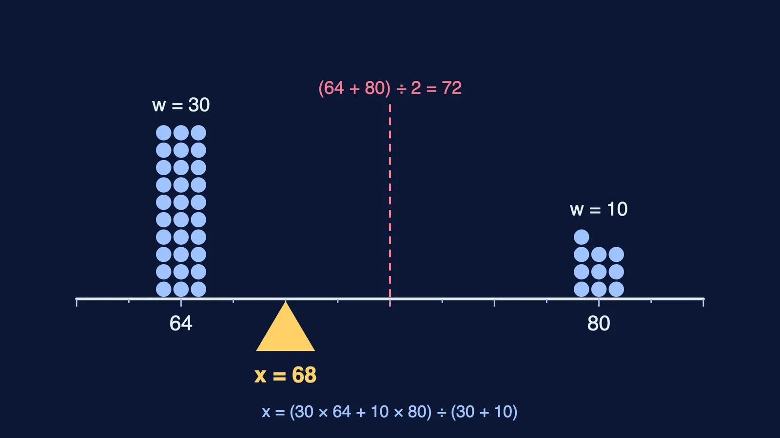
Worked example. Section A has 30 students averaging 64; Section B has 10 averaging 80. Combined average = (64 × 30 + 80 × 10) ÷ 40 = 2,720 ÷ 40 = 68, the balance point in the diagram above, not (64 + 80) ÷ 2 = 72. If Section B then leaves, (68 × 40 − 80 × 10) ÷ 30 = 1,920 ÷ 30 = 64. Backwards: 5 litres of pani is 9% spice. How much water y brings it to 6%? Spice = 0.09 × 5 = 0.45 L, so 0.45 ÷ (5 + y) = 0.06, 5 + y = 7.5 and y = 2.5 litres.
Watch for: adding averages and dividing when the groups differ in size; and forgetting that added water is 0% spice but still adds to the total.
What do stacked and 100% stacked bar charts show?
One calculation turns a stacked bar chart into a 100% stacked one (NCERT Chapter 10).
Percentage share of a part = (part ÷ total of its bar) × 100.
In a 100% stacked bar, the shares in each bar add up to 100%.
Stacked can become 100% stacked, but not back: the totals are lost.
Worked example. Bus X carries 60 students, 24 of them from Class 9; Bus Y carries 30, 18 of them from Class 9. Shares: 24 ÷ 60 × 100 = 40% and 18 ÷ 30 × 100 = 60%. Bus Y has the bigger share; Bus X carries more Class 9 students.
Watch for: comparing amounts across bars on a 100% chart. It shows shares only.
What are the probability formulas in Class 9?
Chapter 7 gives a scale, two formulas and sample spaces (NCERT Chapter 7).
Probability scale: 0 ≤ P(E) ≤ 1, where P(E) is the probability of event E; 0 means impossible and 1 means certain.
Experimental probability = number of times the event occurred ÷ total number of trials. It is also called the relative frequency.
Theoretical probability: P(A) = number of favourable outcomes ÷ number of possible outcomes. Condition: every outcome is equally likely.
Sample space S: the list of all possible outcomes, each listed once. Its sample size is n(S).
An event is a subset of the sample space.
Estimate for a population ≈ estimated probability × population size, if the sample represents the population.
Worked example. You roll a die 120 times and get a 5 on 26 rolls. Experimental P(5) = 26 ÷ 120 ≈ 0.217; theoretical P(5) = 1 ÷ 6 ≈ 0.167. The gap tends to shrink as trials increase, which the chapter calls the Law of Large Numbers. For E = "a prime number", E = {2, 3, 5} and P(E) = 3 ÷ 6 = 0.5. If 14 of 40 surveyed students cycle, a school of 900 has about 0.35 × 900 = 315 cyclists.
Watch for: an answer outside 0 to 1, which means a counting slip; and the gambler's fallacy: after three 6s, a fair die still gives a 6 with probability 1/6.
Our Mathematics of Maybe key terms explains sample space, event and relative frequency in plain words.
How to revise this formula sheet
Write the weighted mean from memory.
Before any average, ask: are the groups the same size?
Do one mixture problem forwards and one backwards.
Write the sample space before any fraction, and label answers experimental or theoretical.
If a method keeps going wrong, the Fermi Problem Library has worked problems with a step-by-step solver that explains the reasoning rather than printing an answer.