
On this page
This sheet covers Chapter 9, Differential Equations, of the NCERT Class 12 Mathematics Part II textbook (Reprint 2026-27), in the chapter's order. Each formula and worked example below was checked with SymPy.
The CBSE Mathematics curriculum for 2026-27 lists the scope: definition, order and degree, general and particular solutions, separation of variables, homogeneous equations of first order and first degree, and linear equations dy/dx + py = q or dx/dy + px = q. Forming a differential equation by eliminating arbitrary constants is not in the 2026-27 syllabus and has no section in the 2026-27 chapter, so it is left out here.
For the step-by-step answer layout and a revision plan, read our differential equations Class 12 board exam guide.
What are order, degree and the general solution?
Symbols: x is the independent variable, y the dependent variable, y′ = dy/dx, y″ = d²y/dx².
Order = the order of the highest derivative present.
Degree = the highest power (a positive integer) of the highest-order derivative, defined only when the equation is a polynomial in its derivatives.
A solution is any function that satisfies the equation.
General solution: contains as many arbitrary constants as the order of the equation.
Particular solution: the general solution with the constants fixed by given conditions, so it has no arbitrary constants.
Worked example: (d²y/dx²)³ + 4(dy/dx)⁵ − y = 0 has order 2 and degree 3. For y″ = 9y, the function y = C₁e^(3x) + C₂e^(−3x) works for every C₁, C₂, and the two constants match order 2, so it is the general solution. With y(0) = 2 and y′(0) = 0 you get C₁ + C₂ = 2 and 3C₁ − 3C₂ = 0, so C₁ = C₂ = 1 and the particular solution is y = e^(3x) + e^(−3x).
Watch for: an equation such as d²y/dx² + cos(dy/dx) = 0 has order 2 but no degree, because a derivative sits inside cos. Write "not defined", not 1.
Variables separable: when can you split x and y?
Symbols: g(x) is a function of x only, h(y) a function of y only, C an arbitrary constant.
Form: dy/dx = g(x) · h(y).
Condition: h(y) ≠ 0 when you divide by it.
Method: (1/h(y)) dy = g(x) dx, then ∫ dy/h(y) = ∫ g(x) dx + C.
Result: H(y) = G(x) + C, where H and G are antiderivatives of 1/h(y) and g(x).
Worked example: dy/dx = (2x + 1)/(3y²) with y(0) = 2. Separate: 3y² dy = (2x + 1) dx. Integrate: y³ = x² + x + C. Put x = 0, y = 2: C = 8, so y³ = x² + x + 8.
Watch for: ∫ dy/y = log|y|, with the modulus. Write + C once, as soon as you integrate.
Homogeneous equations: how does y = vx work?
Symbols: λ is any nonzero constant, n the degree of homogeneity, v a new variable.
Homogeneous function of degree n: F(λx, λy) = λⁿ F(x, y). Example: x² − 3xy has degree 2.
Homogeneous differential equation: dy/dx = F(x, y), where F is homogeneous of degree zero, so F(x, y) = g(y/x).
Substitution: y = vx, so dy/dx = v + x dv/dx.
Then x dv/dx = g(v) − v, and, where g(v) − v ≠ 0, ∫ dv/(g(v) − v) = ∫ dx/x + C. Replace v by y/x at the end.
If the equation is dx/dy = h(x/y), use x = vy, so dx/dy = v + y dv/dy.
Worked example: dy/dx = (x² + 3y²)/(2xy) with y(1) = 1. Replacing x, y by λx, λy leaves the right side unchanged: degree zero. Put y = vx: g(v) = (1 + 3v²)/(2v), so g(v) − v = (1 + v²)/(2v). Then ∫ 2v/(1 + v²) dv = ∫ dx/x, which gives log(1 + v²) = log|x| + log K (K > 0). Near the point (1, 1), x > 0, so 1 + y²/x² = Kx and x² + y² = Kx³. Put (1, 1): K = 2, so x² + y² = 2x³.
Watch for: dy/dx becomes v + x dv/dx, not dv/dx. Leaving the final answer in v loses the last step.
Linear equations: what is the integrating factor?
Symbols: P and Q are constants or functions of x only; P₁ and Q₁ are constants or functions of y only; I.F. is the integrating factor.
Form dy/dx + Py = Q: I.F. = e^(∫P dx), and the general solution is y · I.F. = ∫ (Q × I.F.) dx + C.
Form dx/dy + P₁x = Q₁: I.F. = e^(∫P₁ dy), and the general solution is x · I.F. = ∫ (Q₁ × I.F.) dy + C.
Before reading off P, make the coefficient of dy/dx equal to 1.
Useful identity: e^(log f(x)) = f(x) for f(x) > 0, so P = 1/x gives I.F. = x.
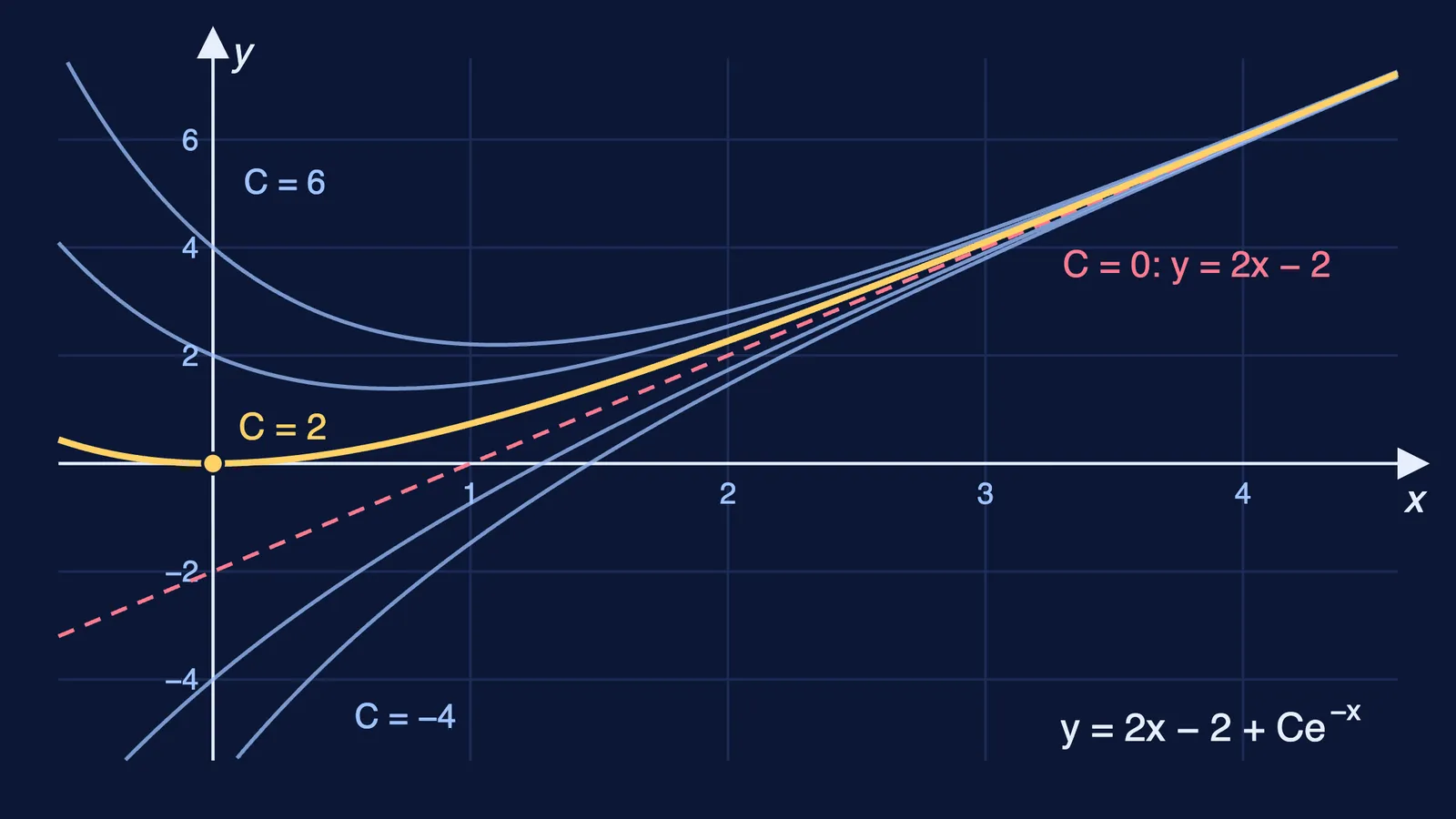
Worked example: dy/dx + y = 2x with y(0) = 0. Here P = 1 and Q = 2x, so I.F. = e^x. Then y e^x = ∫ 2x e^x dx = 2e^x(x − 1) + C, which gives y = 2x − 2 + Ce^(−x). Put x = 0, y = 0: C = 2, so y = 2x − 2 + 2e^(−x). The graph at the top shows this family; the condition picks the gold curve.
Watch for: divide by the integrating factor only after the + C is in place. Writing y = 2x − 2 + C misses the e^(−x) on the constant.
If a step in your working keeps going wrong, the Fermi Problem Library has worked problems with a step-by-step solver that explains the reasoning rather than printing an answer.
How to revise this formula sheet
Sort before you solve: label ten mixed equations as separable, homogeneous or linear, then solve them.
Rewrite the three methods from memory on one side of a page, including the conditions (h(y) ≠ 0, degree zero, P and Q in x only), then check against this sheet.
Check every answer by differentiating it back into the equation; this catches lost constants and sign slips.
Practise the integrals the linear method throws up, such as ∫ x e^x dx and ∫ e^x sin x dx; our integrals Class 12 board exam guide covers integration by parts.