On this page
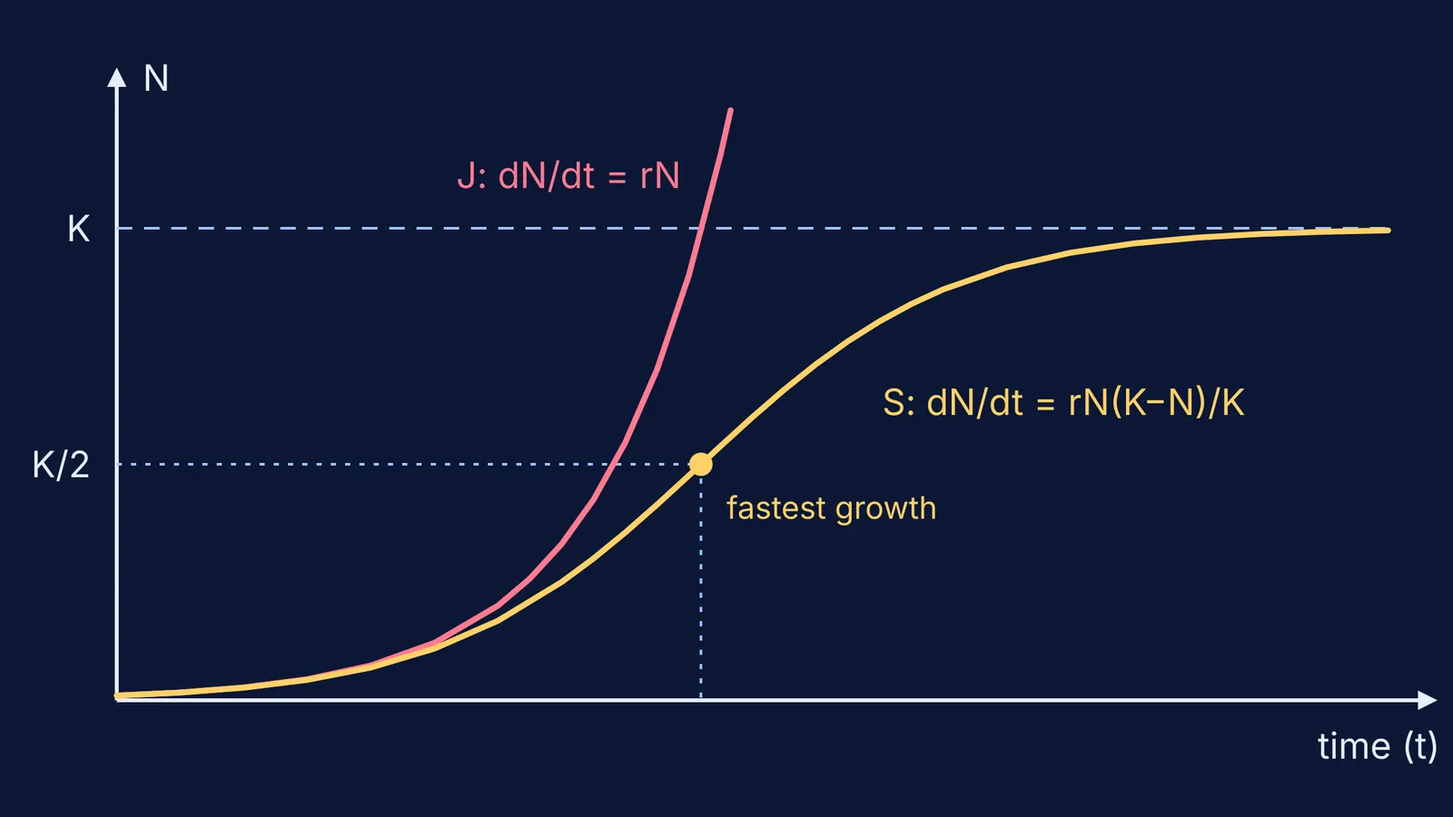
Start a simulated habitat with ten organisms. If food and space never run out, the count shoots up in a J. If they do run out, it bends into an S and settles at a ceiling. Each shape comes from one short equation, so you can predict most of what happens before you press play.
What is the difference between exponential and logistic growth?
The NCERT Class 12 Biology chapter Organisms and Populations writes exponential growth as dN/dt = rN, where r is the intrinsic rate of natural increase: the per-capita birth rate minus the per-capita death rate. Its integral form is N = N₀e^(rt). Plot N against time and you get a J-shaped curve.
The same NCERT chapter gives a sense of scale for r: 0.015 for the Norway rat, 0.12 for the flour beetle, and 0.0205 for India's human population in 1981.
Logistic growth adds a brake. NCERT calls it Verhulst-Pearl logistic growth and writes it as dN/dt = rN(K − N)/K. The plot is a sigmoid (S-shaped) curve: a lag phase, then acceleration, then deceleration, and finally an asymptote at the carrying capacity. Because resources for most animal populations are finite and become limiting sooner or later, NCERT considers the logistic model the more realistic one.
What is carrying capacity in population growth?
Carrying capacity (K) is the maximum population size a particular environment can support (OpenStax Biology 2e).
Read the brake term (K − N)/K as the fraction of room left. As OpenStax explains, when N is small this fraction is close to 1, so growth is nearly exponential. As N gets large, it falls towards 0 and growth slows sharply or stops. Real populations don't always sit neatly on K: OpenStax notes that wild sheep and harbour seal populations exceed it for short periods and then fall below it.
When is a logistic population growing fastest?
At half the carrying capacity. The growth rate rN(K − N)/K is a downward parabola in N, zero at N = 0 and at N = K, so it peaks midway, at N = K/2, where it equals rK/4. Under logistic assumptions, growth is fastest at half the carrying capacity, the idea behind maximum sustainable yield in fisheries.
That point is also where the S changes from curving up to curving down. Below K/2 the curve gets steeper, and above K/2 it flattens. An easy slip is to say growth is fastest at K. At K it is actually zero.
Worked example: what should you predict before you press play?
Set the simulation to N₀ = 10, r = 0.5 per day and K = 1,000. Then use the two equations from the NCERT chapter to write these predictions down first:
Doubling time without limits: ln 2 / r, about 1.4 days.
J-curve at day 10: 10 × e^5, about 1,484, which is already past K. By day 20 it is about 2.2 lakh.
S-curve at day 10: 1,000 / (1 + 99e^−5), about 600.
Fastest growth: at N = 500, around day 9.2 (t = ln 99 / r), at a rate of rK/4 = 125 per day.
Early on, the curves are nearly the same: at day 4, the J gives about 74 and the S about 69.
By day 20, the S-curve is at about 996, within half a percent of K.
If the simulation disagrees, find out why before moving on. A model that updates in steps rather than continuously can behave differently; our guide to what physics simulations can and cannot show covers such mismatches.
What should you change in the simulation next?
Change one setting at a time and predict before each run:
Double r and keep K the same. The S gets steeper, it still levels off at the same K, and the time to reach K/2 halves.
Halve K. The ceiling and the fastest-growth point both halve, but the early, nearly exponential part barely changes.
Start above K, say N₀ = 1,500. The logistic equation gives a negative dN/dt, so the population falls back to K.
Plot dN/dt against N. You should see a hump that peaks at K/2.
To turn real birth and death counts into rates, work through how to calculate birth rate, death rate and population growth. For the wording traps examiners set on this chapter, see how to avoid assertion-reason traps in ecology.
The Fermi Simulation Lab has interactive simulations for ideas that are easier to see than to read, so you can keep up the predict-then-check habit across topics. If the K/2 derivation is the shaky part, Fermi's AI tutor can work out what you already know and build a plan for the session.
Next time you see an S-curve, find K, mark K/2 and point to the steepest part before reading the caption.