On this page
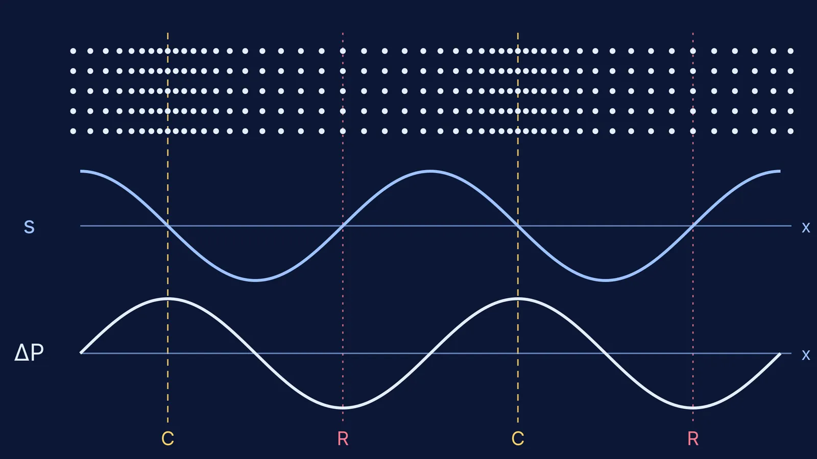
The textbook picture of sound is a row of dots, bunched in places, with a wavy line under it. That wavy line can mean two different things, and mixing them up is an easy slip. Here is how to build the picture in three layers, then test it.
What is actually moving in a longitudinal sound wave?
In a sound wave, air molecules oscillate in simple harmonic motion about their equilibrium positions, parallel to the direction the wave travels, as OpenStax University Physics, section 17.1 describes. Each molecule stays near its home position. Only the pattern travels.
That pattern is a train of compressions (high-pressure regions) and rarefactions (low-pressure regions) moving out with the same frequency as the source, as the same OpenStax section explains.
The speed of sound in air at 20 °C is 343 m/s, according to OpenStax section 17.2.
The motions are tiny: at the threshold of hearing, molecules vibrate over less than one molecular diameter (OpenStax section 17.3). Every diagram, including ours above, exaggerates them.
How do you visualise a longitudinal wave step by step?
Build it one layer at a time, top to bottom.
Particles. Draw a row of evenly spaced dots. That is still air.
Displacement. Choose a curve s(x) and shift each dot sideways by s. Above the axis means pushed forward (in the direction the wave travels). Below means pushed back. Now the dots are uneven.
Pressure. Find where the dots are crowded and mark that as high pressure. Mark the gaps as low pressure. Then sketch ΔP(x).
Step 2 is where students go wrong. The s graph looks like a transverse wave, but it only records sideways shifts. The dots never move up or down.
Where do compressions sit on the displacement graph?
Predict first: on the s graph, does a compression sit at a crest, at a trough or somewhere else?
Look at a point where s is zero and the curve is falling. Just to its left, s is positive, so those particles have moved forward, towards the point. Just to its right, s is negative, so those particles have moved back, also towards the point. Particles from both sides crowd in, while the particle at the point itself has not moved. That is a compression.
Where s is zero and rising, the neighbours have moved apart, which makes a rarefaction. At a crest or a trough, neighbouring particles have shifted the same way by almost the same amount, so the spacing (and the pressure) is close to normal.
Why are pressure and displacement 90° out of phase?
Pressure depends on how squashed the air is. That depends on how displacement changes from one particle to the next, which is the slope of the s graph, not its height. A steep falling slope means strong crowding. A flat crest means no crowding.
OpenStax writes displacement as s(x, t) = smax cos(kx ∓ ωt + φ) and the pressure change as ΔP = ΔPmax sin(kx ∓ ωt + φ). Cosine and sine are a quarter cycle apart, so the pressure graph sits a quarter wavelength away from the displacement graph. The two sizes are linked too: ΔPmax = βk·smax, where β is the bulk modulus and k is the wave number (OpenStax section 17.3).
A worked example you can check
Take a 343 Hz tone in air at 20 °C, where sound travels at 343 m/s (OpenStax section 17.2). The wavelength is λ = v/f = 343/343 = 1 m.
Compressions are 1 m apart, with a rarefaction halfway between them, 0.5 m from each.
At this instant, the particle exactly at a compression has zero displacement.
The most displaced particles sit 0.25 m on either side of a compression, where the pressure is atmospheric.
A quarter period later (about 0.73 ms), the pattern has moved 0.25 m forward.
Common slips: calling a crest of the s graph a compression, and thinking the particles travel with the wave.
How can you test your picture in a simulation?
A static diagram freezes one instant. In a moving one, write each prediction down before you press play:
Freeze it. Find a compression in the particle row, then the same x on both graphs. Is s zero and ΔP at its peak?
Follow one dot. As a compression passes, it should be at home and moving forward fastest; as a rarefaction passes, at home and moving back.
Double the frequency. Compressions should sit twice as close while the speed stays the same, since v = √(B/ρ) depends on the medium (OpenStax section 17.2).
The Fermi Simulation Lab has interactive simulations for ideas that are easier to see than to read, and the same predict-first habit works there. If bulk modulus is the shaky part, the Fermi Concept Library gives each physics concept its own lesson.
The same predict-first habit works with our Doppler effect simulation guide. For a transverse contrast, see how wave speed on a string changes with tension, and for where these pressure swings end up, how a microphone turns sound waves into electric current.