

On this page
Sound waves travel through air as longitudinal pressure variations of alternating compressions and rarefactions, as detailed in our guide to displacement and pressure waves in sound. When these oscillating pressure fronts strike a surface, they impart mechanical force. A microphone captures this vibration and converts it into a matching electrical signal.
Every microphone uses a lightweight diaphragm that moves when sound strikes it. The method used to translate that movement into voltage splits audio physics into two core architectures: electromagnetic induction and variable capacitance.
How does a dynamic microphone use magnetic induction?
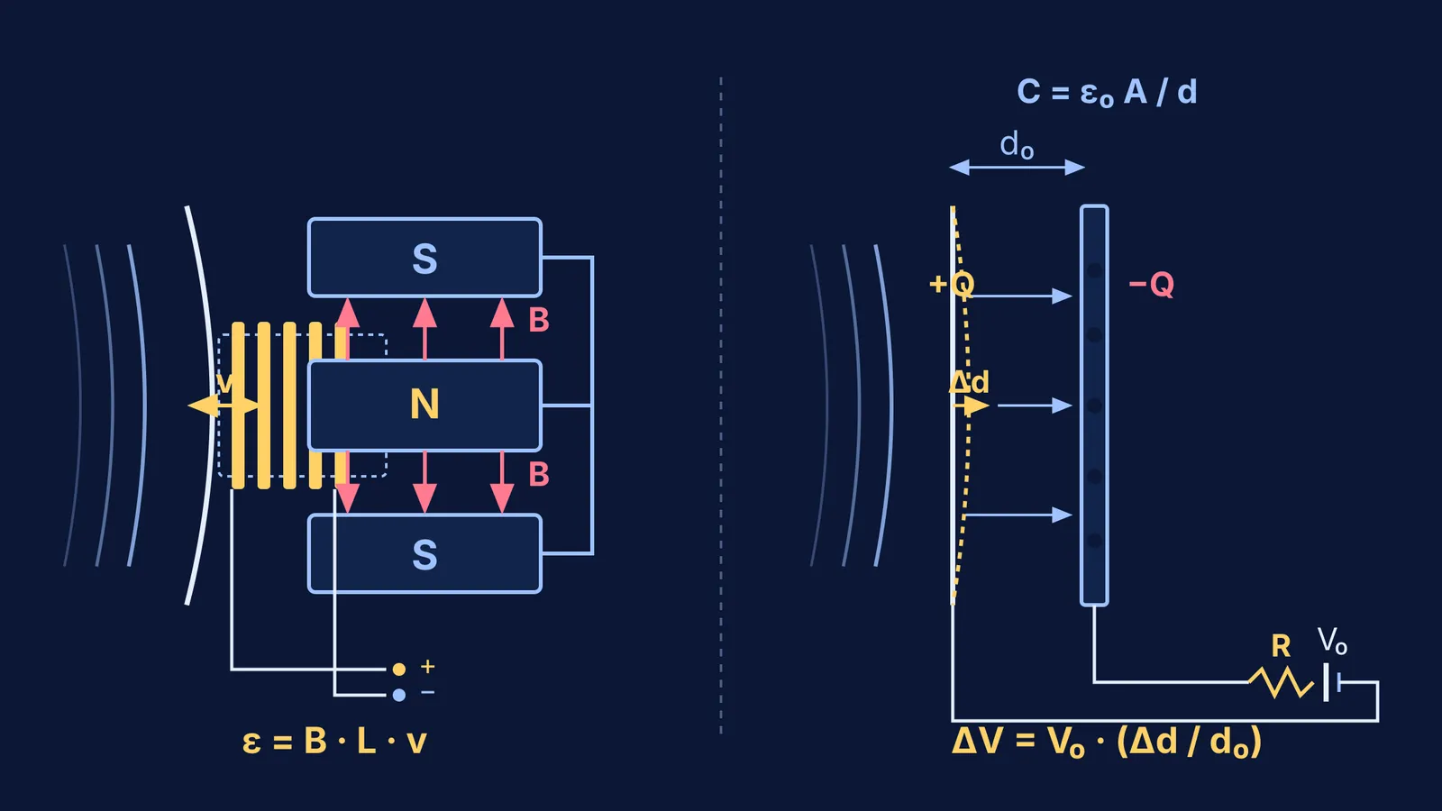
In dynamic microphones, electricity is generated by moving a conductor through a magnetic field. In 1931, Bell Telephone Laboratories researchers Edward Christopher Wente and Albert L. Thuras introduced the modern moving-coil microphone in The Journal of the Acoustical Society of America. Their design fixed a cylindrical coil of fine copper wire to a diaphragm, suspending it within the radial field of a permanent magnet.
When sound waves push the diaphragm, the attached voice coil moves along the magnetic gap with instantaneous velocity v = dx/dt. Because the conductor cuts magnetic flux lines at right angles, a motional electromotive force (EMF) is induced across the coil according to Faraday's law:
ε = B × L × v
Here, B is magnetic flux density in teslas, L is total wire length in the field (L = 2πr × N for N turns of radius r), and v is coil velocity. In accordance with Lenz's law, as analyzed in our guide to Faraday's and Lenz's laws, the induced current creates a field opposing the motion. Because voltage depends on velocity rather than static displacement, dynamic microphones are velocity-sensitive transducers that require no external power.
How does a condenser microphone turn capacitance into voltage?
Condenser microphones rely on electrostatic capacitance. In 1917, E. C. Wente published the operational principles of the condenser microphone in Physical Review, creating an instrument for uniform sound measurement.
The capsule forms a parallel-plate capacitor. A flexible conductive diaphragm sits parallel to a rigid metal backplate across a microscopic air gap d₀, typically 20 to 50 micrometres wide. The resting capacitance C₀ follows:
C₀ = ε₀ × A / d₀
where A is diaphragm area and ε₀ ≈ 8.854 × 10⁻¹² F/m is the permittivity of free space. A direct current (DC) polarizing voltage V₀ charges the plates through a large bias resistor R, usually 100 MΩ to 1 GΩ.
This high resistance controls the charging rate. As explored in our guide to RC circuits: charging, discharging and the time constant, the time constant τ = R × C dictates how fast charge moves. With C ≈ 50 pF and R = 1 GΩ, τ equals 0.05 seconds, creating a low-frequency cutoff f = 1 / (2πRC) of roughly 3.2 Hz. Because audible sound oscillates much faster than this rate, charge Q remains constant during vibration.
When sound displaces the diaphragm by Δd, the gap becomes d₀ + Δd. Because Q = C × V is fixed, voltage varies inversely with capacitance:
V(t) = Q / C(t) = Q × (d₀ + Δd) / (ε₀ × A)
Subtracting the DC bias yields the signal voltage:
ΔV = V₀ × (Δd / d₀)
Because output voltage tracks displacement Δd rather than coil speed, condenser microphones are displacement-sensitive transducers.
How do dynamic and condenser output voltages compare?
Consider both transducers responding to a standard sound pressure of 1 Pascal (94 dB sound pressure level), as standardized in audio engineering references such as Analog Devices' microphone sensitivity guide:
Dynamic capsule calculation:
Coil: N = 40 turns, radius r = 5 mm (0.005 m), wire length L = 40 × 2π × 0.005 m ≈ 1.257 m.
Magnetic flux density: B = 0.60 T.
Diaphragm velocity: v = 2.5 × 10⁻³ m/s.
Peak induced EMF:
ε = B × L × v = 0.60 T × 1.257 m × (2.5 × 10⁻³ m/s) ≈ 1.89 mV.
Condenser capsule calculation:
Plate area: A = 3.14 × 10⁻⁴ m² (radius 10 mm).
Rest separation: d₀ = 25 μm = 2.5 × 10⁻⁵ m.
Baseline capacitance: C₀ = (8.854 × 10⁻¹² F/m × 3.14 × 10⁻⁴ m²) / (2.5 × 10⁻⁵ m) ≈ 111 pF.
Polarizing voltage: V₀ = 48 V.
Acoustic deflection: Δd = 10 nm = 1.0 × 10⁻⁸ m.
Peak signal voltage:
ΔV = 48 V × (1.0 × 10⁻⁸ m / 2.5 × 10⁻⁵ m) = 19.2 mV.
The condenser capsule generates roughly ten times more voltage than the dynamic design, but requires an active buffer circuit before driving an audio cable.
How can you connect microphone physics to exam problems?
Microphone transducers unify three core syllabus topics:
Motional EMF from electromagnetic induction.
Parallel-plate capacitance and charge conservation in electrostatics.
The RC time constant in alternating current circuits.
When seeing how magnetic flux lines cut a moving loop or how electric charge remains frozen during fast oscillations feels abstract, interactive models make the mechanics tangible. In the Fermi Simulation Lab, you can explore interactive simulations for the ideas that are easier to see than to read, manipulating moving conductors in magnetic fields and adjusting capacitor plate geometry to see how induced EMF and field lines respond in real time. If you are solving numerical problems on induction or RC circuits, the Fermi Problem Library provides worked problems with a step-by-step solver that explains the reasoning rather than printing an answer.


