
On this page
You know that √4 = 2. Now try √4.1 without a calculator. It must be a little more than 2, but how much more? A tangent line answers that in four lines of working, and checking the answer shows you what a derivative really means.
Before you read on, write down a guess. Then check whether your guess is too big or too small. Making a prediction first gives you something to check.
What is the tangent line approximation?
The linear approximation of a function f at x = a is L(x) = f(a) + f′(a)(x − a), which is the equation of the tangent line at that point (OpenStax Calculus Volume 1, section 4.2). The same textbook gives the idea in one sentence: for x near a, the graph of the tangent line is close to the graph of f. Its own worked example uses the tangent at 9 to estimate √9.1 as about 3.0167, and the true value is about 3.0166.
The trick is to pick an anchor point a where you know everything exactly, then walk a short distance along the straight tangent instead of the curve.
How do you approximate the square root of 4.1 with a tangent?
Choose the nearest perfect square: a = 4, so f(4) = √4 = 2.
Differentiate: f′(x) = 1/(2√x), so f′(4) = 1/4.
Write the tangent: L(x) = 2 + (x − 4)/4.
Substitute x = 4.1: L(4.1) = 2 + 0.1/4 = 2.025.
So √4.1 ≈ 2.025. If you want to see why a slope of 1/4 is the right one, our post on the derivative as the slope of a tangent builds that picture step by step.
Is the tangent estimate too big or too small?
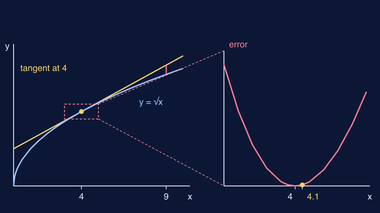
Too big, slightly. The graph of y = √x bends downward (it is concave down), so its tangent lies above it. Wikipedia's article on linear approximation states the rule: if f is concave down between a and x, the linear approximation is an overestimate; if concave up, an underestimate.
A calculator gives √4.1 = 2.0248457 to seven decimal places. The tangent's 2.025 is high by about 0.00015, which is roughly 0.0076% of the true value. Rounded to four significant figures, the true value is 2.025, exactly what the tangent gave.
You can even predict the size of the error. Taylor's theorem says the error is f″(c)/2 × (x − a)² for some c between a and x (OpenStax Calculus Volume 2, section 6.3). For √x, f″(x) = −1/(4x√x), which has size at most 1/32 between 4 and 4.1. So the error is at most (1/64) × (0.1)² = 0.00015625. The real error, 0.0001543, sits just under that bound.
What happens when you zoom in, or move further away?
Here is the same tangent, L(x) = 2 + (x − 4)/4, tested at four points (true values from a calculator):
x = 4.01: tangent 2.0025, true 2.0024984, error about 0.0000016
x = 4.1: tangent 2.025, true 2.0248457, error about 0.00015
x = 5: tangent 2.25, true 2.2360680, error about 0.014
x = 9: tangent 3.25, true 3, error 0.25
Look at the first two lines. The step shrank ten times, from 0.1 to 0.01, and the error shrank about a hundred times. That is the (x − a)² in Taylor's theorem at work: halve the distance and the error drops to roughly a quarter.
This is what "zoom in" means. Magnify the graph around (4, 2) far enough and the curve and its tangent become impossible to tell apart. Zoom out to x = 9 and they have clearly parted. That is why, for √9.1, the OpenStax example anchors at 9 rather than 4: always anchor at the nearest point you know.
Zooming is easier to see than to read, and the Fermi Simulation Lab has interactive simulations for ideas like this.
How can you practise this in five minutes?
Use the same predict-then-check routine on each question:
Write the nearest perfect square and its root.
Predict: will the tangent be too big or too small? (For square roots, always too big.)
Find the slope 1/(2√a) and the tangent value.
Estimate the error with h² ÷ (8a√a).
Only now check with a calculator.
Try √9.2 (tangent gives 3.0333; true value about 3.03315) and √15.9 (tangent at 16 gives 3.9875; true value about 3.98748). Notice that √15.9 sits below its anchor, yet the tangent still overshoots: concavity, not direction, decides.
For other routes to the same number, compare this with our guides to estimating square roots without a calculator and the Babylonian guess-and-average method. If you get stuck on a step, the Fermi Problem Library has worked problems with a step-by-step solver that explains the reasoning rather than printing an answer.