
On this page
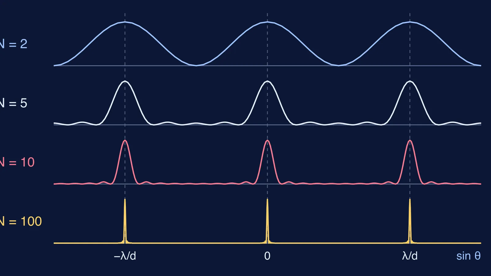
A grating gives thin, bright lines on a dark background, while Young's two slits give broad, soft stripes. Adding slits does not move the bright lines at all. It only squeezes them. Here is why, using phasor sums for 2, 5, 10 and 100 slits at the same spacing.
Where do the bright lines of a grating appear?
A diffraction grating is a surface ruled with a large number of evenly spaced parallel lines, where the untouched gaps act as slits, and OpenStax University Physics notes that a grating can have over 1,000 lines per millimetre. The bright lines, called principal maxima, appear where d sin θ = mλ, with m = 0, ±1, ±2 and so on. Why a CD shows rainbow colours applies it to a real grating.
Notice what is missing: N, the number of slits. At a principal maximum, neighbouring slits differ in path by a whole number of wavelengths, so every slit arrives in step. So with d fixed, the lines stay put for any N.
The phase difference between neighbouring slits is φ = 2π d sin θ / λ, and the principal maxima sit at φ = 0, ±2π, ±4π (University of Illinois Physics 214 lecture notes).
How do phasors explain sharper lines?
Treat each slit's wave as an arrow, a phasor, of the same length. To add N waves, place the arrows head to tail, each turned by φ from the one before. Intensity is the square of the final arrow's length (Illinois lecture notes).
At a principal maximum, φ = 0 and all N arrows point the same way. The total is N arrows long, so the peak intensity is N² times that of one slit.
Step a little off the maximum and the arrows start to curl into an arc. The total gets shorter.
The first dark point comes when the arrows curl all the way round into a closed polygon. That needs Nφ = 2π, so φ = 2π/N, which gives θ ≈ λ/(Nd) beside the central maximum.
The same notes show that between two neighbouring principal maxima there are N − 1 zeros and N − 2 weaker secondary maxima, and that the peak width goes as 1/N. OpenStax's multiple-slit section adds the energy argument: the total light is unchanged, so narrower maxima must be brighter.
What do 2, 5, 10 and 100 slits look like?
Take d = 2 µm (500 lines per mm) and λ = 500 nm. The first-order line is at sin θ = λ/d = 0.25, about 14.5°, for every value of N. Near the central maximum, the half-width to the first dark point is λ/(Nd) = 0.25/N radians. Applying the Illinois formulas to each case:
N = 2: about 7.2°. Peak 4 times one slit. One zero between maxima, no secondary maxima.
N = 5: about 2.9°. Peak 25 times. Four zeros and three small bumps between maxima.
N = 10: about 1.4°. Peak 100 times. Nine zeros and eight tiny bumps.
N = 100: about 0.14°. Peak 10,000 times. Ninety-nine zeros; most of the 98 bumps are too small to show on a sketch.
Why does a tiny step off the maximum matter more with more slits?
The full result is I = I₁ × [sin(Nφ/2) / sin(φ/2)]², from the Illinois notes. Turn each arrow 20° from the last, so the chain bends through Nφ in all, and compare with each grating's own peak:
N = 2: Nφ = 40°. The two arrows are only 20° apart and nearly line up: 97% of the peak.
N = 5: Nφ = 100°. The arc bends: 78%.
N = 10: Nφ = 200°. The arrows curl past a half-circle: 32%.
N = 100: Nφ = 2,000°, more than five full loops. The arrows almost cancel: 0.32%.
A step that barely dims a double slit makes a 100-slit grating nearly dark. That is why a grating can separate colours whose lines lie close together.
How should you practise sketching N-slit patterns?
A ten-minute pencil routine:
Write φ = 2π d sin θ / λ and mark φ = 0 and 2π.
Draw N equal arrows in a line for φ = 0; the total is N.
Redraw them turned by 2π/N each and check they close into a polygon.
Sketch: lines in fixed places, N − 1 zeros, N − 2 bumps.
Repeat for the next N and say what changed and what did not.
Real slits have a width too. HyperPhysics explains that the observed pattern is the multiple-slit interference expression multiplied by the single-slit diffraction expression. Our post on counting fringes inside the central diffraction maximum shows how that envelope works.
To start from two slits, try predicting and measuring fringe width in a Young's double slit simulation. For more ideas that are easier to see than to read, the Fermi Simulation Lab has interactive simulations to explore.