
On this page
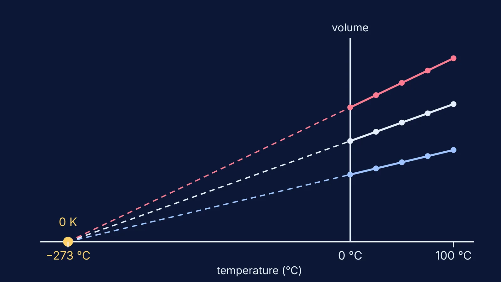
If you plot the volume of a gas against its temperature in degrees Celsius, keeping the pressure and the amount of gas fixed, you get a straight line that does not pass through the origin. Extend that line to the left and it reaches zero volume near −273 °C. That crossing point is absolute zero, and you can find it yourself with a gas simulation, a ruler and five readings.
What does Charles's law say?
Charles's law says that the volume of a gas is directly proportional to its thermodynamic (kelvin) temperature, as long as the amount of gas and the pressure stay constant, according to LibreTexts' ChemPRIME chapter on Charles's law/09%3A_Gases/9.08%3A_Charles's_Law). In symbols, V = kT. The same source dates the first quantitative studies of this behaviour to Jacques Charles in 1787.
NASA Glenn Research Center's page on the law gives a clean example: a gas at 4.0 cubic metres and 300 K, cooled to 225 K at constant pressure, shrinks to 3.0 cubic metres, because 4/300 equals 3/225.
The catch is the word kelvin. On the Celsius scale the volume still rises in a straight line, but the line has an intercept, so volume is not proportional to the Celsius number. That intercept is what the graph lets you find.
Why does the volume–temperature line hit zero at −273 °C?
NIST states that one Celsius degree is an interval of 1 K and that zero degrees Celsius is 273.15 K. NIST also notes that 0 K is commonly called absolute zero.
Put those together with V = kT. If T = t + 273.15, where t is the Celsius reading, the volume is V = V₀(1 + t/273.15), with V₀ the volume at 0 °C. Each degree of warming adds 1/273.15 of the 0 °C volume. Set V to zero and you get t = −273.15 °C.
This does not depend on which gas you use or how much of it. LibreTexts/09%3A_Gases/9.08%3A_Charles's_Law) shows two different samples whose lines, extended to very low temperatures, both cross the temperature axis at −273 °C.
Real gases never reach zero volume: the same LibreTexts chapter/09%3A_Gases/9.08%3A_Charles's_Law) notes that hydrogen at 1 atm liquefies at −253 °C.
How do you extrapolate a Charles's law graph to absolute zero?
LibreTexts/09%3A_Gases/9.08%3A_Charles's_Law) does this with hydrogen data: it extends the lines beyond the measured points. Use any gas simulation that holds pressure constant while you change temperature. Then:
Fix the pressure and the number of particles.
Set the temperature to 0, 25, 50, 75 and 100 °C. At each one, wait for the volume to settle and write it down.
Plot volume on the y-axis and Celsius temperature on the x-axis. Let the x-axis run from about −300 °C to 100 °C, so there is room to extend.
Draw the best straight line through your points, then continue it as a dashed line until it meets V = 0.
Read the crossing point, or calculate it: crossing temperature = −(volume at 0 °C) ÷ slope.
For a worked example, suppose your readings, rounded to two decimal places, are 2.00, 2.18, 2.37, 2.55 and 2.73 L at 0, 25, 50, 75 and 100 °C. (These are what an ideal gas with 2.00 L at 0 °C would give, using the relation above.)
Slope from the end points: (2.73 − 2.00) ÷ 100 = 0.0073 L per °C.
Crossing temperature: −2.00 ÷ 0.0073 ≈ −274 °C.
A least-squares line through all five points gives a slope of 0.00732 L per °C and a crossing of about −273.2 °C.
Now the trap. Use only the 50, 75 and 100 °C readings and the slope becomes (2.73 − 2.37) ÷ 50 = 0.0072 L per °C. The line then crosses at 50 − 2.37 ÷ 0.0072 ≈ −279 °C. Rounding to hundredths of a litre became a six-degree miss, because you stretched the line over 300 degrees past your data. Spread your readings as wide as the simulation allows, and use all of them.
What should you test once the line works?
Treat the simulation as a place to make predictions, then check them:
Double the number of particles. Prediction: a steeper line, same crossing point.
Raise the pressure. Prediction: smaller volumes, same crossing point.
Replot the same data with kelvin on the x-axis. Prediction: the line now passes through the origin.
If you want to run this instead of only reading about it, the Fermi Simulation Lab has interactive simulations for ideas that are easier to see than to read. Fermi's AI tutor can run the simulation with you and check your understanding as it goes, so a wrong prediction becomes a question, not a dead end.
Next, see why the coefficient of volume expansion of an ideal gas equals 1/T, why Carnot efficiency needs temperatures in kelvin, or try Boyle's law with a syringe, plotting P against 1/V.