
On this page
When a cyclone forms over the Bay of Bengal, far from the reach of coastal radar, forecasters rely mainly on a satellite parked over the equator. India's INSAT weather satellites watch the same face of the Earth all day, and India Meteorological Department (IMD) forecasters use their pictures to find a storm's centre, judge its strength and work out where it is heading.
Why do INSAT satellites stay over India?
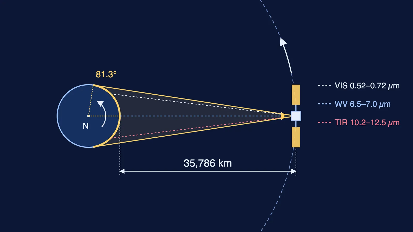
INSAT-3D was launched on 26 July 2013 and sits in geostationary orbit at 82° East, according to ISRO's INSAT-3D page.
Its altitude is about 35,786 km above the equator, says MOSDAC, ISRO's meteorological data centre (MOSDAC: INSAT-3D spacecraft). At that height one orbit takes as long as one turn of the Earth, so the satellite seems to hang still. Our post on why geostationary satellites sit 36,000 km high shows how that height falls out of Newton's law of gravitation.
A satellite in low orbit passes over a storm only a few times a day; a geostationary one can photograph it again and again. INSAT-3DR, at 74° East, is "identical to INSAT-3D in terms of Sensors and products" (MOSDAC: INSAT-3DR). INSAT-3DS, launched on 17 February 2024, carries a 6-channel imager and a 19-channel sounder to "augment the Meteorological services" alongside them (ISRO: GSLV-F14/INSAT-3DS mission).
What do the six imager channels see?
Each channel is a narrow slice of the spectrum, listed on MOSDAC's INSAT-3D payload page:
Visible (0.52–0.72 µm), 1 km pixels: sunlight reflected off clouds. The sharpest picture, but daytime only.
Shortwave infrared (1.55–1.70 µm), 1 km: reflected sunlight at a longer wavelength.
Middle infrared (3.80–4.00 µm), 4 km: gives "night time pictures of low clouds and fog", says ISRO's INSAT-3DR page.
Water vapour (6.50–7.00 µm), 8 km: water vapour absorbs and re-emits strongly here, so the image maps moisture high in the atmosphere, even where there is no cloud.
Two thermal infrared bands (10.2–11.2 and 11.5–12.5 µm), 4 km: heat given off by cloud tops and the ground. Colder tops are higher, and high, cold tops mean deep storms.
Thermal infrared works day and night, which is why an IMD training presentation calls IR imagery "available for continuous monitoring round the clock" (IMD: Tropical cyclone, intensification and movement-Dr-M-Mohapatra.pdf)).
How is a cyclone's track forecast from satellite images?
The same IMD presentation sets out the chain forecasters follow (IMD slides-Dr-M-Mohapatra.pdf)).
Fix the centre. Early on, it is the middle of the low cloud lines; once spiral bands form, forecasters fit a logarithmic spiral to them; once an eye forms, the eye is the centre. Over open sea, the typical satellite location error is about 55 km.
Estimate the strength. The Dvorak technique turns cloud patterns into a Current Intensity (CI) number. In IMD's table, CI 3.0 means about 45 knots, CI 4.0 about 65 knots and CI 5.0 about 90 knots.
Read the steering winds. The deep-layer flow around a storm accounts for up to 80% of its motion; the beta effect, from the Coriolis force changing with latitude, adds 10–20%. Water vapour images show the troughs and ridges that do the steering.
Run the models. Forecasters weigh tracks from several weather models and issue a forecast with a cone of uncertainty.
Our post on how IMD forecasts the weather covers the wider routine, and close to the coast Doppler weather radar takes over as the main tool for fixing the centre.
Try it: can you forecast a track from two positions?
The IMD slides include a worked example of CLIPER, a simple model that blends persistence (keep doing what you were doing) with climatology (what storms in that month usually do) (IMD slides-Dr-M-Mohapatra.pdf)).
Past position: 13.5°N, 88.0°E. Present position, 12 hours later: 14.5°N, 90.5°E.
That is 1.0° north and 2.5° east. One degree of latitude is about 111 km; at 14°N a degree of longitude is about 111 × cos 14° ≈ 108 km.
So the storm moved about 111 km north and 269 km east: roughly 290 km in all, or 24 km/h.
Persistence alone puts it at 16.5°N, 95.5°E after 24 hours. Climatology says 17.1°N, 90.4°E. CLIPER averages them: 16.8°N, 93.0°E.
The two answers sit hundreds of kilometres apart, which is why forecasters lean on steering winds and models rather than a straight line.
If geostationary orbits are hard to picture, the Fermi Simulation Lab has interactive simulations for ideas that are easier to see than to read, and the Fermi Concept Library gives every physics concept its own lesson.