
On this page
Most students meet integration twice: once as "reverse differentiation" and once as "area under a curve". Few are shown why these are the same thing. One picture links them: a growing area, and the thin strip it gains each time you nudge its right-hand edge. Once you see the strip, the fundamental theorem of calculus stops being a formula to memorise.
What is the area function A(x)?
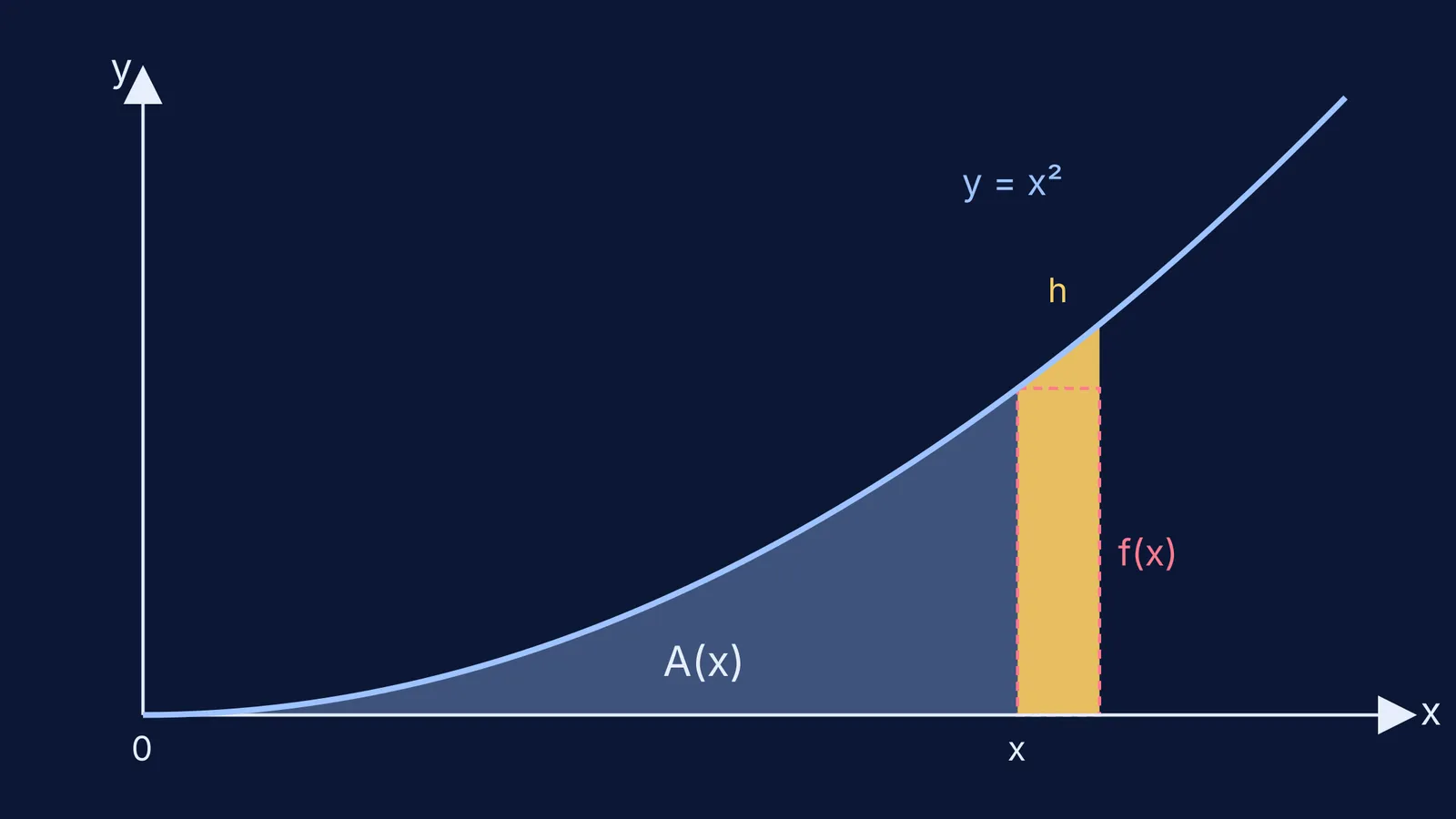
Take a curve y = f(x) that stays above the x-axis, and fix a starting point a. Now let the right-hand edge slide. The area function A(x) is the area under the curve from a up to x. It is a function like any other: give it an x, and it returns an area.
The free OpenStax textbook Calculus Volume 1 writes this as F(x) = ∫ₐˣ f(t) dt, and states the first part of the fundamental theorem: if f is continuous on [a, b], then F′(x) = f(x).
Why does the area grow at a rate equal to the curve's height?
Push the edge from x to x + h, where h is tiny. The new area is the old area plus a thin strip (yellow in the diagram above). That strip is almost a rectangle of height f(x) and width h, so A(x + h) − A(x) ≈ f(x) × h. The geometric proof on Wikipedia's fundamental theorem page uses exactly this strip.
Divide both sides by h and you get (A(x + h) − A(x)) / h ≈ f(x). The left side is the slope of A over a short step. As h shrinks, the curved top of the strip matters less and less, and in the limit the approximation becomes exact. That limit is the derivative, so A′(x) = f(x).
In words: the area grows at a rate equal to the curve's height. Where the curve is tall, each step adds a lot of area. Where the curve touches the axis, the area barely grows.
So why does integration give the area?
Now run it backwards. A(x) is a function whose derivative is f. Any antiderivative F you find with the usual rules also has derivative f. Two functions with the same derivative on an interval differ only by a constant, so A(x) = F(x) + C. At x = a the area is zero, so C = −F(a), and the area from a to b is A(b) = F(b) − F(a).
That is the second part of the theorem as OpenStax states it: if f is continuous on [a, b] and F is any antiderivative of f, then ∫ₐᵇ f(x) dx = F(b) − F(a). The constant cancels, which is why you never carry +C in a definite integral. If the "same derivative, differ by a constant" step feels shaky, read why the derivative of a constant is zero.
The same OpenStax section notes that Newton and Leibniz, among others, worked out this link between derivatives and integrals in the late 1600s and early 1700s.
Worked example: area under y = x² from 0 to 2
Estimate with rectangles. Split [0, 2] into four strips of width 0.5. Left-edge heights 0, 0.25, 1 and 2.25 give 3.5 × 0.5 = 1.75. Right-edge heights 0.25, 1, 2.25 and 4 give 7.5 × 0.5 = 3.75. The true area lies between them.
Use the theorem. An antiderivative of x² is x³/3, so the area is 2³/3 − 0 = 8/3 ≈ 2.667, which sits between 1.75 and 3.75 as it must.
Check the strip picture. With A(x) = x³/3, push from x = 2 by h = 0.1: A(2.1) − A(2) = (9.261 − 8)/3 ≈ 0.4203, against a rectangle of f(2) × h = 4 × 0.1 = 0.4.
Shrink the step. With h = 0.01 the strip is (8.120601 − 8)/3 ≈ 0.0402003, against 0.04. Divided by h, the growth rates are about 4.203 and 4.02003, closing in on f(2) = 4.
Which exam mistakes does this picture prevent?
Area below the axis. There f(x) is negative, so each strip subtracts. The integral gives signed area; for the actual area, split at the roots, as shown in why you split the interval at roots.
Differentiating an integral with a variable limit. d/dx ∫ₐˣ f(t) dt is just f(x), straight from the strip. If the upper limit is g(x), the edge moves at rate g′(x), so the answer is f(g(x)) × g′(x).
Treating integration as a bag of rules. The same height-times-width strip gives the familiar circle formula in deriving πr² with a definite integral.
If a step in problems like these trips you up, the Fermi Problem Library has worked problems with a step-by-step solver that explains the reasoning rather than printing an answer. To revisit limits, derivatives and definite integrals one idea at a time, the Fermi Concept Library gives each concept its own lesson and its place in the map.
Next time you write ∫, picture the yellow strip: height f(x), width h, added again and again.