
On this page
The common-emitter (CE) transistor practical asks you to draw two kinds of graph and pull two numbers out of them: input resistance and current gain. Here are the circuit, the readings and a worked calculation to check your record against.
First, check that it is on your list. The CBSE Physics curriculum for 2025-26 limits Class 12 semiconductor theory to diodes, and its only electronics experiment is the diode I-V curve. The transistor experiment still appears in college labs and online Virtual Labs, so check your own board's or university's current list.
What is the circuit for transistor CE characteristics?
The IIT Bombay Virtual Lab experiment uses a BC547B n-p-n transistor, a breadboard, 1 kΩ and 100 kΩ resistors, a 0-100 µA ammeter, a 0-10 mA ammeter, a 0-30 V DC supply and a multimeter. The emitter is shared by both circuits, hence "common emitter". Wire two loops:
Input loop: base supply, a series resistor (usually the 100 kΩ) and the microammeter to the base; a voltmeter across base and emitter reads VBE.
Output loop: collector supply, a series resistor (usually the 1 kΩ) and the milliammeter to the collector; a voltmeter across collector and emitter reads VCE.
Emitter: connected to the negative terminal of both supplies for an n-p-n transistor. For p-n-p, reverse both supplies and both meters.
The Virtual Lab defines the active region, where the transistor amplifies, as the state in which the base-emitter junction is forward biased and the base-collector junction is reverse biased.
How do you plot the input characteristics (IB vs VBE)?
Set VCE to a fixed value and write it above the table.
Raise VBE from zero in small steps.
At each step, record VBE and IB, and reset VCE if it has drifted.
Plot IB against VBE.
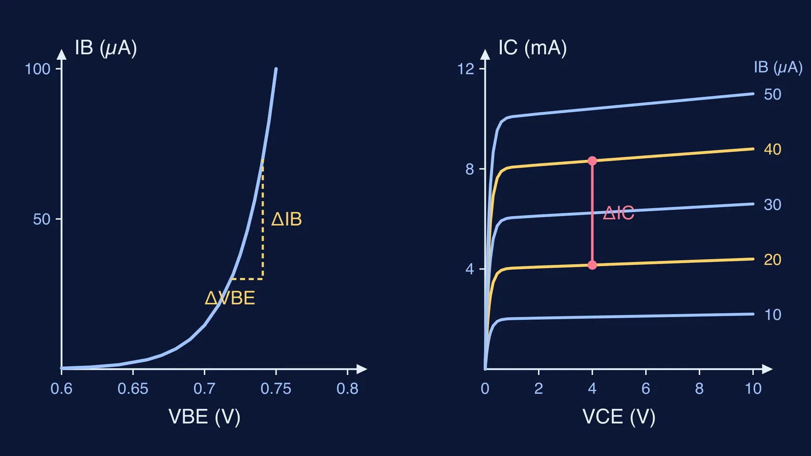
The Virtual Lab notes that this curve resembles a forward-biased diode's: IB stays near zero, then rises rapidly after the cut-in voltage. Take closely spaced readings above it, where you will measure the slope.
How do you plot the output characteristics (IC vs VCE)?
Set IB to a fixed value, say 20 µA.
Raise VCE from zero in small steps and record IC, holding IB constant.
Repeat for two or three more values of IB.
Plot all the curves on one graph and label each with its IB.
Each curve rises steeply at very small VCE (saturation, where both junctions are forward biased), then flattens into a nearly level line (the active region). The flat part is where you read the gain.
How do you find input resistance and current gain from the graphs?
The Virtual Lab gives the dynamic input resistance as ΔVBE/ΔIB at constant VCE and the dynamic output resistance as ΔVCE/ΔIC at constant IB. It defines β as the ratio IC/IB; from graphs you usually find the ac current gain, βac = ΔIC/ΔIB at constant VCE. Here is a worked example using sample readings from the diagram above.
Input resistance. On the input curve, VBE = 0.72 V gives IB = 30 µA, and VBE = 0.74 V gives IB = 70 µA.
ΔVBE = 0.74 - 0.72 = 0.02 V
ΔIB = 70 - 30 = 40 µA = 40 × 10⁻⁶ A
ri = 0.02 / (40 × 10⁻⁶) = 500 Ω
Current gain. Draw a vertical line at VCE = 4 V. It cuts the IB = 20 µA curve at IC = 4.16 mA and the IB = 40 µA curve at IC = 8.32 mA.
ΔIC = 8.32 - 4.16 = 4.16 mA
ΔIB = 40 - 20 = 20 µA
βac = 4.16 × 10⁻³ / (20 × 10⁻⁶) = 208
Output resistance. On the IB = 40 µA curve, IC rises from 8.32 mA at VCE = 4 V to 8.64 mA at VCE = 8 V, so ro = 4 / (0.32 × 10⁻³) = 12.5 kΩ.
If the arithmetic is where you lose marks, the Fermi Problem Library has a step-by-step solver that explains the reasoning, so you can check each conversion, not just the answer.
What mistakes cost marks in this practical?
The Virtual Lab gives the BC547's typical maximum current rating as 100 mA. Keep well below that, and run through this checklist before you hand in your record:
VCE held constant for every input reading, and written on the graph.
µA and mA converted to amperes before you divide.
Gain read from a change (ΔIC/ΔIB), unless the question asks for the dc value IC/IB.
Slopes taken from the steep part of the input curve and the flat part of the output curves.
Supply polarity checked against the transistor type before you switch on.
Our guide to writing precautions and sources of error turns this list into record-book sentences. The Zener diode reverse characteristic practical uses the same plot-then-read-the-slope routine, and for the junction behaviour behind the curves, see how to ask AI about forward and reverse bias.
For the physics behind each curve, the Fermi Concept Library covers every concept in physics.