
On this page
The Zener practical asks you to push a diode into reverse breakdown on purpose, which can damage an ordinary diode unless the current is limited.
Check your syllabus first. CBSE's Class 12 physics curriculum for 2026-27 lists the I-V curve of a p-n junction diode in forward and reverse bias, not a Zener experiment. If your lab sets the Zener version, use this guide; the circuit and graph skills carry over to the p-n junction experiment.
What happens in a Zener diode in reverse bias?
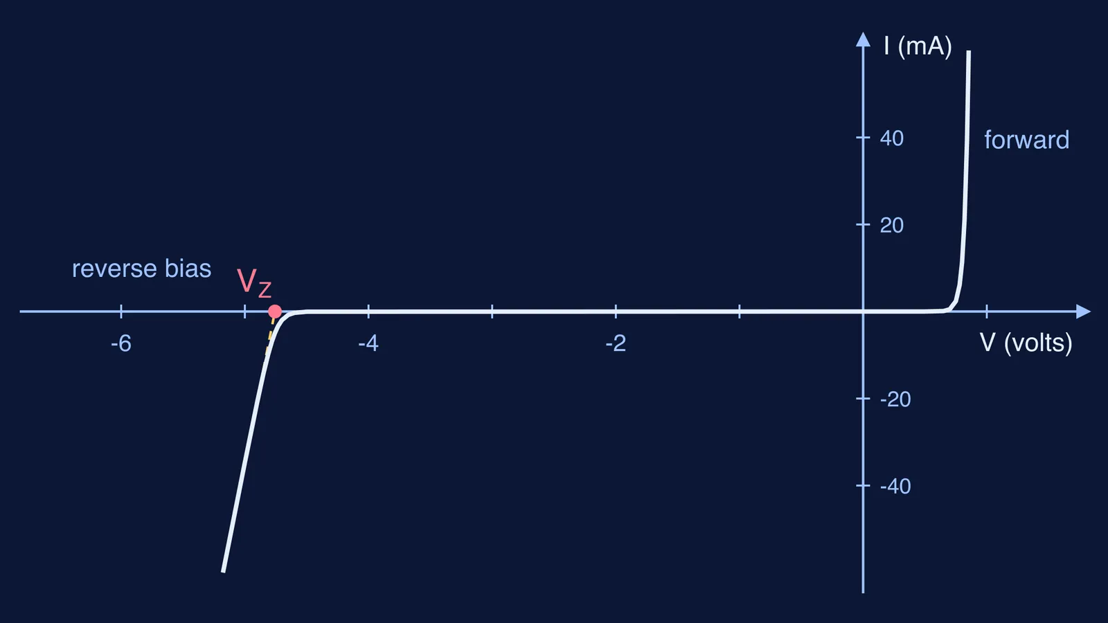
The NISER lab manual on diode characteristics describes a Zener diode as a heavily doped p-n junction. In reverse bias almost no current flows until the reverse voltage reaches the breakdown voltage; then the current rises sharply while the voltage across the diode stays nearly constant.
In a heavily doped junction the depletion layer is narrow, and the field is strong enough to break covalent bonds and free electron-hole pairs: this is Zener breakdown. In a lightly doped junction, breakdown happens through collisions instead, which is avalanche breakdown. For why doping sets the width, read how doping affects depletion region width.
If that picture is shaky, the Fermi Concept Library gives every physics concept its own lesson, so you can revisit the unclear one before the viva.
How do you connect a Zener diode in reverse bias?
The NISER manual uses a 0-30 V DC supply, a 1 kΩ current-limiting resistor and two multimeters. Wire it like this:
Supply positive to the resistor, the resistor to the milliammeter, and the milliammeter to the diode's cathode (the end with the band).
The diode's anode back to the supply negative.
The voltmeter directly across the diode, not across the supply.
Set the meter ranges before you switch on; how to choose ammeter and voltmeter ranges covers the method.
Is a 1 kΩ resistor safe for a Zener diode?
Take a 1N4733A. Vishay's datasheet gives its Zener voltage as 5.1 V at a test current of 49 mA, with a tolerance of ±5%, a maximum regulator current of 178 mA and a maximum power dissipation of 1300 mW at 25 °C.
At the full 30 V, the resistor drops 30 − 5.1 = 24.9 V, so the current is 24.9 V ÷ 1000 Ω = 24.9 mA, well under 178 mA.
The diode dissipates 5.1 V × 24.9 mA ≈ 0.13 W, far below 1.3 W.
The resistor dissipates 24.9 V × 24.9 mA ≈ 0.62 W. If your resistor is rated 0.25 W, it will overheat. Keep the supply below about 20 V, where the resistor takes (20 − 5.1)² ÷ 1000 ≈ 0.22 W, or ask for a higher-wattage resistor.
How do you take the readings?
Following the NISER procedure:
Start at 0 V and raise the supply in 0.5 V steps. Record the supply voltage, the voltage across the diode and the current.
At first the current is tiny. Vishay lists a maximum leakage of 10 µA at 1 V for the 1N4733A, so use the most sensitive current range.
When the current starts climbing quickly, you have reached breakdown. Switch to 0.1 V steps and take at least six readings here.
Switch off between sets, and do not let the resistor or diode run hot.
For the write-up, see how to write precautions and sources of error in practicals.
How do you read the breakdown voltage from the graph?
Plot current against diode voltage, with reverse values on the negative axes so the curve sits in the third quadrant. Then:
Draw one straight line through the steep points after the knee.
Extend it until it meets the voltage axis. That intercept is your breakdown voltage, Vz.
Pick two points on the steep part and find the dynamic resistance, r = ΔV/ΔI, as the NISER manual defines it. For example, if the diode voltage moves from 4.90 V to 4.97 V while the current goes from 10 mA to 20 mA, r = 0.07 V ÷ 0.010 A = 7 Ω.
The Vishay datasheet specifies the 1N4733A's 5.1 V ±5% (about 4.85 V to 5.36 V) at 49 mA, with a typical dynamic resistance of 7 Ω there and up to 550 Ω at 1 mA, near the knee. Your circuit reaches only about 25 mA, so your r will usually come out a little larger than 7 Ω. A line of slope 7 Ω through 5.1 V at 49 mA meets the voltage axis near 4.76 V, so an intercept roughly between 4.5 V and 5.4 V points to a healthy diode and a good graph.
When you move on to numericals built on this curve, the Fermi Problem Library has worked problems with a step-by-step solver that explains the reasoning rather than printing an answer.