
On this page
Chapter 7 of Ganita Manjari, the new NCERT Class 9 maths book for 2026-27, teaches you to put a number on "maybe". It is short, but the ideas are worth getting exactly right.
What does Chapter 7 of Ganita Manjari cover?
Ganita Manjari Part I is NCERT's first edition, dated April 2026 (NCERT, Part I front matter). Its foreword says Chapter 7 introduces randomness, empirical and theoretical probability, tables and tree diagrams, with an eye on experiments and simulation.
Inside the chapter, randomness means you know every possible result but not which comes next, and every probability sits on a scale from 0 (impossible) to 1 (certain).
How do you find experimental and theoretical probability?
The chapter's key move is keeping these two apart. Experimental probability is the number of times an event happened divided by the total number of trials (Ganita Manjari, Chapter 7). Theoretical probability is the number of favourable outcomes divided by the number of possible outcomes, assuming each outcome is equally likely (same source).
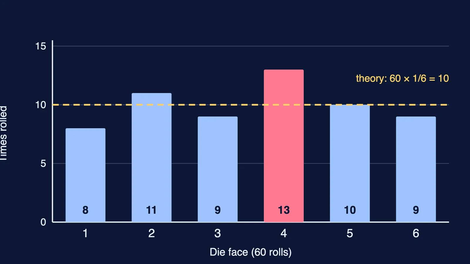
Worked example 1 (experiment). Suppose you roll a die 60 times and record the counts in the chart above: 8, 11, 9, 13, 10 and 9 for faces 1 to 6.
Experimental P(4) = 13 ÷ 60 ≈ 0.217, or about 21.7%.
Theoretical P(4) = 1 ÷ 6 ≈ 0.167, or about 16.7%.
Check: the six relative frequencies add to 60 ÷ 60 = 1, as explained in why the probabilities of all elementary events add up to 1.
The two answers differ, and that is normal. The chapter notes that with few trials the experimental value can stray from the theoretical one, and that it tends to move closer as trials increase, which it names the Law of Large Numbers.
Worked example 2 (theory). A bag holds 4 yellow, 5 white and 3 orange marbles, 12 in all. Seven are not white, so P(not white) = 7 ÷ 12 ≈ 0.583. No experiment is needed, because each marble is equally likely to be picked.
Worked example 3 (survey data). In a class of 48, 18 students come by bus, 14 walk, 10 cycle and 6 come by car. The estimated probability that a random student takes the bus is 18 ÷ 48 = 0.375. For a school of 1,200, expect about 0.375 × 1,200 = 450 bus users, if your class is a fair sample of the school. Estimating for a whole population from a smaller group is what the chapter calls sampling.
How do sample spaces and tree diagrams work?
A sample space is the list of every possible outcome, with none missing and none repeated; an event is a subset of it (Ganita Manjari, Chapter 7). Tree diagrams help when an experiment has more than one step.
Worked example 4. Toss a coin, then spin a fair spinner with three equal sectors: red, green, blue. The tree has 2 first branches, each splitting into 3, giving S = {HR, HG, HB, TR, TG, TB}, so n(S) = 6.
P(heads and green) = 1 ÷ 6.
P(tails and not blue) = 2 ÷ 6 = 1/3, from TR and TG.
The Fermi Simulation Lab has interactive simulations for the ideas that are easier to see than to read.
What mistakes cost marks in probability?
Gambler's fallacy. After four sixes in a row, a fair die still gives a six on the next roll with probability 1/6. As the chapter puts it, "the coin has no memory".
Treating unequal outcomes as equal. Two dice give 11 possible sums, but a sum of 2 is not 1/11; only 1 of the 36 equally likely pairs gives it, so it is 1/36. See the probability of a doublet with two dice for the full 36-cell grid, and why two children with at least one boy gives 1/3 for the same trap in a different form.
Mixing the two types. Writing 1/6 when the question asks for the experimental value from your data.
If you keep getting a method wrong, the Fermi Problem Library has worked problems with a step-by-step solver that explains the reasoning rather than printing an answer.
How much is probability worth in CBSE Class 9 2026-27?
In the CBSE 2026-27 Class IX maths curriculum, Unit VI, Statistics and Probability, carries 10 of the 80 theory marks, shared between the Statistics chapter and Introduction to Probability (CBSE curriculum 2026-27). The unit gets 24 periods, and its outcomes include estimating empirical probability from data and using tree diagrams and tables.
A simple plan for the week before your test:
Day 1: write both formulas from memory and do one example of each.
Day 2: draw trees for three two-step experiments.
Day 3: toss a coin 50 times, tally heads after every 10 tosses, and compare each running result with 1/2.
Start the 50 tosses today; watching your running result settle towards 1/2 shows the Law of Large Numbers in your own data.