
On this page
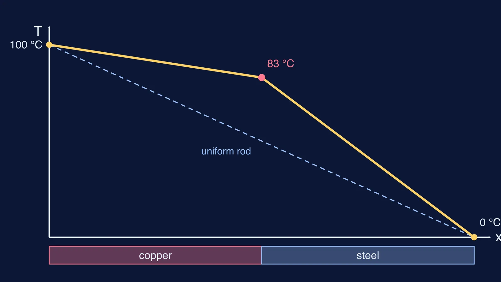
A familiar exam sketch: a rod with one end in boiling water, the other in ice, and the question "draw the temperature along the rod". The answer is short. For one uniform, insulated rod in steady state, the graph is a straight line. For two rods joined end to end, it is two straight lines with a kink at the joint.
Why is the temperature graph of a rod a straight line in steady state?
Start from the conduction law. The rate of heat flow through a slab is P = kA(Th − Tc)/d, where k is the thermal conductivity, A the cross-sectional area and d the thickness, as set out in OpenStax University Physics Volume 2, section 1.6. The same section gives the general form P = −kA(dT/dx), where dT/dx is the temperature gradient. HyperPhysics states the same law in words.
Now apply two facts about steady state:
Temperatures no longer change with time, so no slice of the rod is storing heat.
The sides are insulated, so no heat leaks out sideways.
Together these mean the same heat current H passes through every cross-section. Rearranging the law gives dT/dx = −H/(kA). If k and A are the same all along the rod, the right-hand side is a constant. A constant slope is a straight line. OpenStax says it directly: in steady-state conduction the temperature decreases linearly from the hot end to the cold end.
What happens to the slope where two rods are joined?
At the joint, the heat current still cannot pile up, so H is the same in both rods. Write the law for each part:
k1A1 × (slope in rod 1) = k2A2 × (slope in rod 2)
So the slope in each part is inversely proportional to kA. For rods of equal area, the material that conducts worse has the steeper line. This is easy to get backwards: copper does not "carry more temperature drop"; it needs very little drop to push the same heat through.
Worked example: copper joined to steel
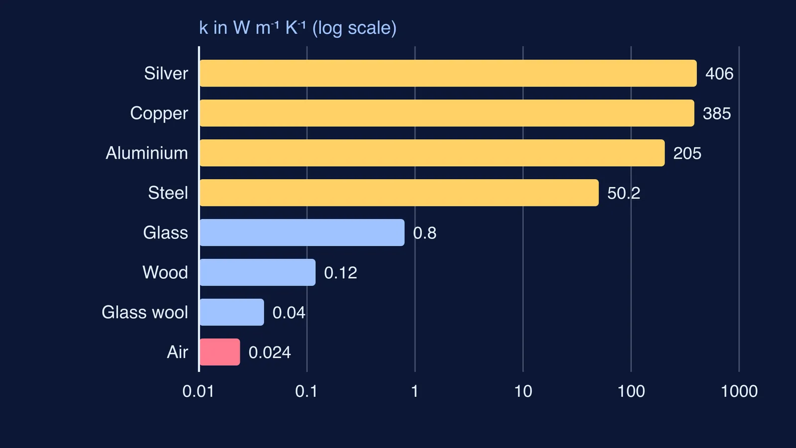
Take a copper rod and a steel rod of equal length L and equal area, joined end to end and insulated. The free copper end is held at 100 °C and the free steel end at 0 °C. Use the conductivities from the OpenStax table: copper 390 W/m·°C and steel (iron) 80 W/m·°C.
Let the junction temperature be T.
Equal heat current: 390 × (100 − T)/L = 80 × (T − 0)/L.
Cancel L and solve: 39000 = 470T, so T ≈ 83.0 °C.
Copper drops 17 °C over length L; steel drops 83 °C over the same length.
Ratio of slopes, steel to copper: 83/17 ≈ 4.9, which matches 390/80. The check works.
So the graph runs almost flat from 100 °C to 83 °C across the copper, then falls steeply to 0 °C across the steel.
Want to test yourself on a second case? OpenStax Example 1.11 joins a steel rod at 100 °C to an aluminium rod at 20 °C, each 0.25 m long and 1.00 cm across, and finds a joint temperature of 41.3 °C and a heat flow of 1.47 W (OpenStax). Before you look, predict which rod has the steeper line.
For more on the junction step itself, see our post on the temperature at the junction of two rods in series. For the formula behind H, read rate of heat flow through a rod and what doubling does.
How do you sketch the temperature graph in an exam?
Use this five-step routine:
Mark the two end temperatures on the T-axis at x = 0 and x = total length.
Find each junction temperature. The quickest way is thermal resistance R = L/(kA): rods in series add like resistors, and each rod takes a share of the total temperature drop in proportion to its R. Our explainer on thermal resistance of rods in series and parallel walks through it.
Join the points with straight segments, one per material.
Check: the steeper segment must belong to the smaller kA.
Allow kinks only at joints. Inside one material, the line stays straight.
Common traps to avoid:
Putting the junction at the average of the end temperatures. That only works when both rods have the same R.
Drawing the good conductor with the steeper slope.
Drawing a smooth curve through the joint instead of a sharp change in slope.
If you want more rods-in-series questions with every step explained, the Fermi Problem Library has worked problems with a step-by-step solver that explains the reasoning rather than printing an answer. If the idea of a temperature gradient itself still feels shaky, look up heat conduction in the Fermi Concept Library, where each concept has its own lesson.