
On this page
A trolley with a pendulum hanging from its roof is released on a smooth incline. What happens to the time period, and which way does the string hang? This JEE favourite looks like it needs heavy algebra. With one pseudo-force and a two-arrow diagram it takes about four lines, and the same method works for lifts and trains too.
Why does the pendulum feel a different gravity in the cart?
The cart is accelerating, so it is not an inertial frame. Inside an accelerating frame you can still use Newton's laws, as long as you add an inertial force. OpenStax University Physics describes these as "fictitious forces that merely seem to arise from motion, because the observer's frame of reference is accelerating or rotating."
For a frame with acceleration a, that pseudo-force on a mass m is −ma: the same size as ma, pointing the opposite way. Add it to real gravity and you get one combined pull, the effective gravity:
g_eff = g − a (as vectors)
The pendulum cannot tell the difference between this and ordinary gravity. It hangs along g_eff and swings as if g had been replaced by |g_eff|.
How do you derive g_eff = g cos θ step by step?
Here is the pseudo-force diagram method, in order.
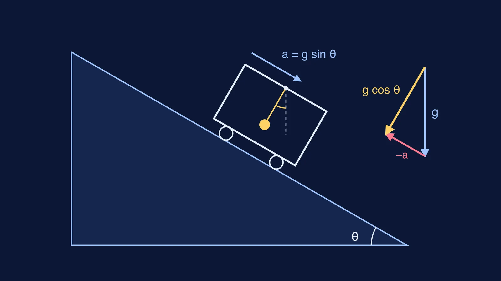
Find the cart's acceleration. On a frictionless incline every object slides with a = g sin θ down the slope, whatever its mass, as OpenStax's section on common forces shows.
Split gravity along the incline axes. Gravity per unit mass has a component g sin θ down the slope and g cos θ into the slope. (If the cos θ part feels shaky, see our post on why the normal force on an incline is mg cos θ.)
Add the pseudo-acceleration −a. That is g sin θ up the slope.
Add the components. Along the slope: g sin θ − g sin θ = 0. Into the slope: g cos θ.
So g_eff = g cos θ, directed perpendicular to the incline. The down-slope part of gravity is used up in accelerating the cart, so only the perpendicular part is left for the pendulum.
Two quick checks catch most sign errors. At θ = 0 you get g cos 0 = g, the ordinary pendulum. At θ = 90° the cart is in free fall and g cos 90° = 0, so the bob floats and there is no oscillation at all.
Which way does the string hang when the cart slides down?
At equilibrium the string lies along g_eff. Since g_eff is perpendicular to the incline, the string rests perpendicular to the slope, making angle θ with the true vertical. Seen from the ground it looks tilted, but relative to the cart's floor it is perfectly upright.
The bob also oscillates about this tilted line, not about the vertical.
What is the time period of the pendulum in the sliding trolley?
For small swings a simple pendulum has T = 2π√(L/g), and OpenStax's pendulum section notes the period is nearly independent of amplitude when the angle is less than about 15°. Replace g with g_eff:
T = 2π√(L / (g cos θ))
Worked example: L = 1.0 m, θ = 30°, g = 9.8 m/s².
On level ground: T₀ = 2π√(1.0/9.8) ≈ 2.01 s.
On the incline: g cos 30° = 9.8 × 0.866 ≈ 8.49 m/s², so T = 2π√(1.0/8.49) ≈ 2.16 s.
Ratio: T/T₀ = 1/√(cos 30°) ≈ 1.07, so the period is about 7% longer.
A pendulum's period depends only on its length and g, not on the bob's mass, as OpenStax College Physics 2e explains. So the mass of the bob, and of the cart, never enters the answer.
How does this compare with other accelerating frames?
The same g − a recipe gives each of these.
Lift accelerating up at a: g_eff = g + a, string vertical, shorter period.
Train accelerating horizontally at a: g_eff = √(g² + a²), string tilted back by tan⁻¹(a/g).
Cart sliding down a smooth incline: g_eff = g cos θ, string perpendicular to the slope.
Cart sliding down a rough incline with coefficient μ: a = g(sin θ − μ cos θ), so g_eff = g cos θ √(1 + μ²), and the string leans forward from the perpendicular by tan⁻¹ μ.
Free fall: g_eff = 0, no oscillation.
If you want to see how the cart itself moves when the incline can also slide, our post on how far a wedge moves as a block slides down uses the same axes. For what real pendulums do as their swings die out, read pendulum damping and amplitude.
If a variant still trips you up, the Fermi Problem Library has worked problems with a step-by-step solver that explains the reasoning rather than printing an answer. For ideas that are easier to see than to read, the Fermi Simulation Lab has interactive simulations.