
On this page
Hold a vibrating tuning fork over a tube with water at the bottom and slowly let the water fall. At one length the tube booms; further down it booms again. A simulation lets you repeat this freely, and the most useful thing to do with it is predict the second length before you find it. The size of the miss shows you the end correction.
What does a resonance tube actually measure?
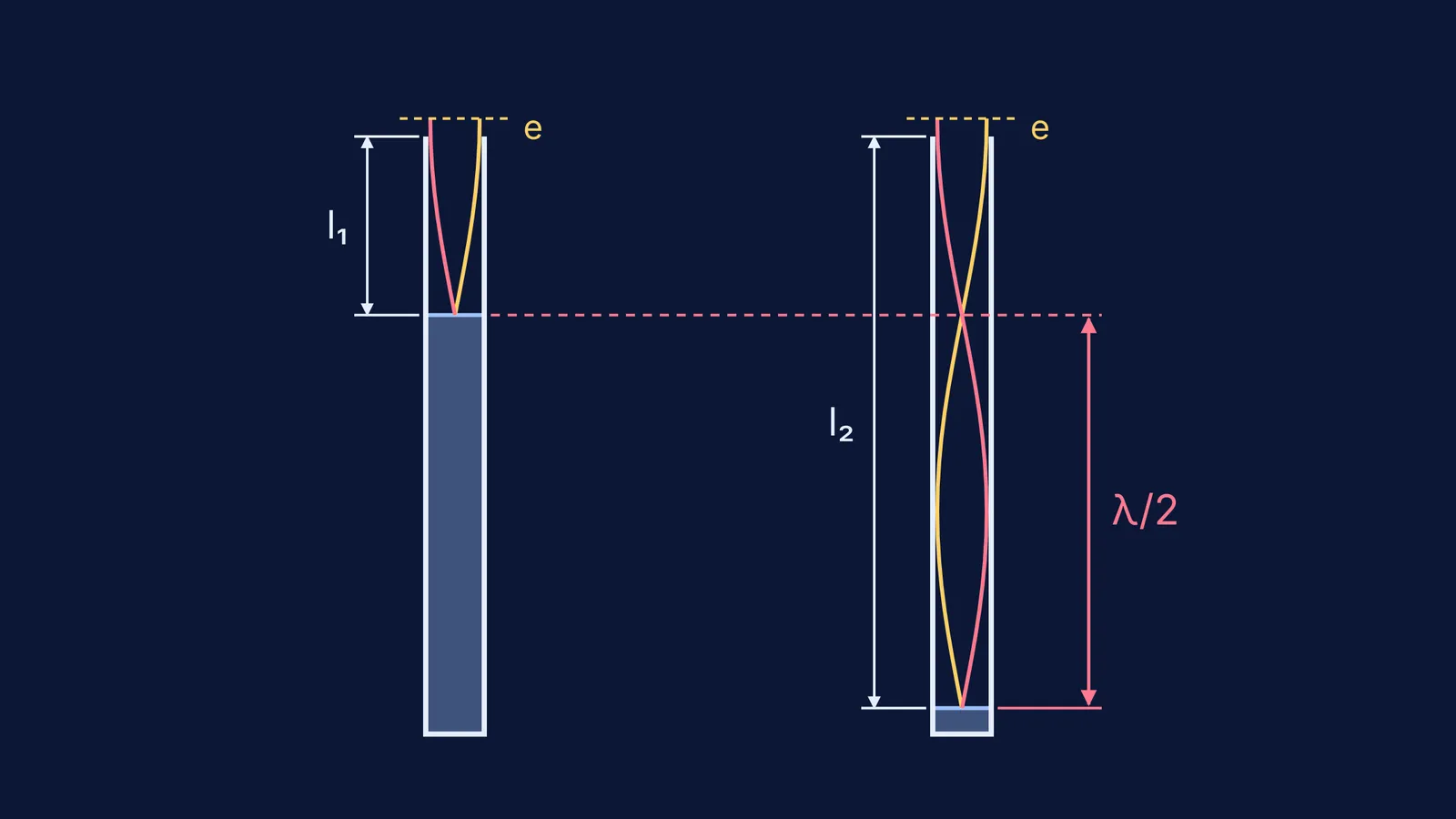
A resonance tube is an air column closed at the bottom by water and open at the top. A tube closed at one end resonates only at its fundamental and odd harmonics, and in the fundamental the wavelength is four times the length of the air column (HyperPhysics, closed tube resonances). The water surface is a displacement node, because air cannot move into the water, and the open end is close to an antinode.
So the tube measures wavelength. Each time the column grows by half a wavelength, a new standing wave fits, and successive resonance lengths differ by λ/2 (Arizona State University resonance tube lab manual). Multiply the wavelength by the fork's frequency and you have the speed of sound. For the same physics run the other way, see how a closed pipe partly filled with water changes frequency.
Where should the second resonance length be?
Here is the prediction game. If the first length l₁ were exactly λ/4, the second, at 3λ/4, would be exactly 3l₁. Write that number down before you move the water.
Then find l₂. It comes out a little longer than 3l₁. The real antinode sits a small distance e above the rim, so the effective lengths are l₁ + e = λ/4 and l₂ + e = 3λ/4. Rearranging gives l₂ = 3l₁ + 2e, and so e = (l₂ − 3l₁)/2.
How do you calculate the speed of sound from two resonance lengths?
The speed of sound in air is about 344 m/s at 20 °C and 331.5 m/s at 0 °C (HyperPhysics speed of sound table). Take a tube 5.0 cm across (radius 2.5 cm), a 512 Hz fork and a 20 °C room. These are the lengths that physics predicts, and what a careful simulation should show:
Raise the water to the top, then lower it slowly. The first resonance comes at l₁ = 15.3 cm.
Predict the second: 3 × 15.3 = 45.9 cm.
Keep lowering. The second resonance comes at l₂ = 48.9 cm, 3.0 cm beyond your prediction.
Speed of sound: v = 2f(l₂ − l₁) = 2 × 512 × 0.336 m = 344 m/s.
End correction: e = (48.9 − 45.9)/2 = 1.5 cm, which is 0.6 of the 2.5 cm radius.
Compare the one-length shortcut: v = 4fl₁ = 4 × 512 × 0.153 m = 313 m/s, about 9% too low.
The subtraction in step 4 cancels e, which is why the two-resonance method beats using l₁ alone. For a route with dust heaps instead of loud notes, see how Kundt's tube measures the speed of sound.
Why does end correction exist?
The air just outside the mouth moves with the air inside, so the tube behaves as if it were slightly longer than it is. HyperPhysics puts the end correction at about 0.6 times the radius of the pipe, added at the open end to get the effective acoustic length (HyperPhysics).
That number has a long pedigree. Harold Levine and Julian Schwinger worked out the radiation of sound from an unflanged circular pipe in Physical Review in 1948 (DOI record). A 1993 Journal of Fluid Mechanics study by Peters, Hirschberg and colleagues gives their value as 0.6133 times the radius for an unflanged pipe with no airflow (abstract).
So a wider tube has a bigger end correction: l₁ shrinks while l₂ − l₁ stays the same.
What should you try next in the simulation?
Change the fork to 384 Hz and predict both lengths first. With the same tube and sound at 344 m/s, the 20 °C value in the HyperPhysics table, expect about 20.9 cm and 65.7 cm.
Raise the temperature. Sound travels faster in warmer air, so both lengths should grow.
If the simulation lets you change the diameter, double it and watch l₁ shrink while l₂ − l₁ holds steady.
If a result surprises you, learn how to ask AI why a simulation surprised you.
Standing waves are easier to see than to read, which is what the Fermi Simulation Lab is for: interactive simulations for ideas like this one. When a JEE problem gives you two resonance lengths and asks for the end correction, the Fermi Problem Library has worked problems with a step-by-step solver that explains the reasoning rather than printing an answer.