
On this page
A scatter plot can look like a clean upward line and still get a correlation coefficient that says almost nothing. The quickest way to feel why is to guess r first, then drag one point and watch it move. Here is a worked example you can do on paper, and a plan for trying it with any tool that lets you drag points.
What does the correlation coefficient r measure?
The Pearson correlation coefficient is r = Sxy / (√Sxx × √Syy), where Sxx and Syy are sums of squared deviations from the mean and Sxy is the sum of cross-products, as set out in the NIST Dataplot reference. A perfect straight-line relationship gives r = +1 (or -1 if it slopes down), and no linear relationship gives r = 0, according to the same NIST page.
Notice the word linear: r measures how well one straight line fits. And because deviations are squared and multiplied, a point far from the others has a large say in the answer.
Predict first: what is r for this scatter plot?
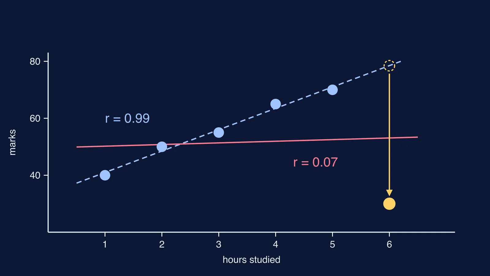
Take a small invented class. Each student records hours studied the evening before a test (x) and their mark out of 100 (y): (1, 40), (2, 50), (3, 55), (4, 65), (5, 70). Before reading on, write down your guess for r.
Now check it by hand:
Means: x̄ = 3, ȳ = 56.
Deviations in x: -2, -1, 0, 1, 2. Deviations in y: -16, -6, -1, 9, 14.
Sxy = 32 + 6 + 0 + 9 + 28 = 75. Sxx = 10. Syy = 570.
r = 75 / √(10 × 570) = 75 / 75.5 ≈ 0.99.
If you guessed 0.8 or 0.9, the answer is a small surprise. Guessing first is not a gimmick. In a 2004 study of physics classroom demonstrations, Catherine Crouch, Eric Mazur and colleagues found that students who only watched a demonstration understood the concept no better than students who never saw it, while students who predicted the outcome before seeing it showed significantly greater understanding (Crouch et al., American Journal of Physics, 2004).
How much can one outlier change the correlation coefficient?
Add a sixth student who was unwell on test day and scored 30. We worked out r for the same six points twice, moving only where that student sits on the x-axis:
Outlier in the middle, at (3, 30): Sxy stays 75, Syy jumps to about 1,133, and r falls from 0.99 to about 0.70.
Outlier at the edge, at (6, 30): Sxy drops to 10, Sxx becomes 17.5, and r falls to about 0.07.
Same unusual score, very different damage. A point at the end of the x-range has the most pull: it can tilt the best-fit line on its own, and r follows.
The statistician Francis Anscombe made the same point in 1973 with four small data sets that share nearly identical means, variances and correlation (r = 0.816) but look completely different when plotted (Anscombe, The American Statistician, 1973). In his third set, ten of the eleven points lie on a straight line and one outlier lowers r from 1 to 0.816; in his fourth, a single point far to the side of the rest produces a high r even though the other points show no relationship (Anscombe's quartet, data and summary). It is the two-dimensional version of how one outlier moves the mean but not the median.
How to try it yourself: a drag-the-point plan
Use any graphing tool that lets you move points and shows r as you drag.
Plot the class above. Guess r, then reveal it.
Add a sixth point mid-range, well below the line. Predict a small or large drop, then check.
Drag it slowly to the right edge. Predict where r falls fastest.
Drag it up onto the trend line, far right. Predict whether r rises or falls.
Start from a shapeless cloud with r near 0 and add one far-away point. Watch how high r climbs.
For each step, write one line: predicted, happened, why.
For other ideas that are easier to see than to read, the Fermi Simulation Lab has interactive simulations you can explore in the same predict-then-check way.
What should you do with an outlier in real data?
Do not delete a point just because it spoils your r. Instead:
Plot the data before you trust r.
Check whether the point is a recording mistake. If it is, fix it and say so.
If it is real, report r with and without it, and explain the difference.
Consider a rank-based measure, where one extreme value carries less weight; see how Charles Spearman introduced rank correlation.
A strong r does not show cause. Scores can also drift back towards average, as in why toppers often score lower next time.
If the arithmetic of Sxy and Syy still feels shaky, the Fermi Problem Library has worked problems with a step-by-step solver that explains the reasoning rather than printing an answer.
Next time you see a correlation in a textbook or a news story, ask for the scatter plot first.