
On this page
Phillip Hagar Smith was a radio engineer at Bell Telephone Laboratories. In January 1939 he published the diagram that now carries his name in Electronics magazine, under the modest title "Transmission line calculator" (Wikipedia biography of Phillip Hagar Smith).
Who invented the Smith chart?
Smith was born on 29 April 1905 in Lexington, Massachusetts, graduated in electrical engineering from Tufts College in 1928 and worked at Bell Labs until he retired in 1970 (Wikipedia biography). He was also an early radio amateur, with the callsign 1ANB.
The problem came first. In 1929 he was working on an antenna connected to the transmitter by a two-wire transmission line, and matching the two was slow work for two people: "One individual moved a cumbersome signal-sensing device along the line at the end of a pole, while a second read the signal through a telescope" (Electronic Design profile of Smith).
His 1939 article opens with the idea behind the whole chart: "Transmission line problems are greatly simplified if the line is terminated by an impedance equal to its characteristic impedance" (the January 1939 article, reprinted by RF Cafe). His cut-out calculator gave the impedance at any point on the line, located the points where the impedance is a pure resistance, and measured line losses on a decibel scale. He published an improved version in the same magazine in January 1944 and a book, Electronic Applications of the Smith Chart, in 1969 (Wikipedia biography).
Others had the same idea: Tōsaku Mizuhashi in Japan independently proposed the chart in 1937, and Amiel R. Volpert in the Soviet Union in 1939; "Smith chart" became the standard name in the Western world by 1950 (Wikipedia: Smith chart).
How does the Smith chart work?
Divide the load impedance Z by the line's characteristic impedance Z0 to get the normalised impedance z = Z/Z0. The reflection coefficient is then Γ = (z − 1)/(z + 1): how much of the wave bounces back, and with what phase (Wikipedia: Smith chart). The Smith chart is a plot of Γ, labelled with z.
A perfect match, z = 1, gives Γ = 0: the centre of the chart.
A short circuit, z = 0, sits at the left edge; an open circuit sits at the right edge.
Any load with positive resistance lands inside the unit circle, because then |Γ| is less than 1.
Constant resistance gives circles; constant reactance gives arcs.
The trick that made it a calculator: moving along a lossless line changes only the angle of Γ, not its size. The impedance repeats every half wavelength, because the angle changes by 2π over a distance of λ/2 (Wikipedia: Smith chart). So one full lap of the chart is half a wavelength of cable, and a long calculation becomes "turn the point around a circle".
If complex division is rusty, our guide to dividing complex numbers using the conjugate covers the step below, and deriving LCR circuit impedance shows where the j comes from.
How do you match a load on a Smith chart?
Suppose an antenna presents Z = 100 + j50 Ω at the end of a 50 Ω cable.
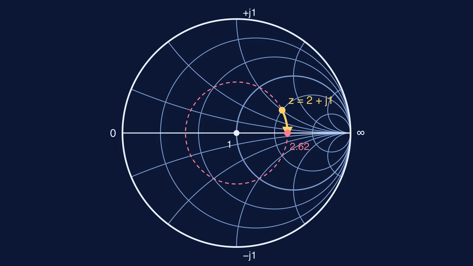
Normalise: z = (100 + j50)/50 = 2 + j1. On the chart this is where the r = 2 circle crosses the x = 1 arc (the yellow dot in the diagram at the top).
Find Γ = (1 + j1)/(3 + j1). Multiply top and bottom by the conjugate 3 − j1 to get (4 + j2)/10 = 0.4 + j0.2. Its size is about 0.447 and its angle about 26.6°.
Draw the circle of constant |Γ| through the point (dashed). Every point along the cable lies on it.
Read the standing wave ratio where the circle crosses the right-hand real axis: (1 + 0.447)/(1 − 0.447) ≈ 2.62, the ratio of largest to smallest voltage on the line.
Rotate clockwise, towards the generator, as Smith's 1939 article does, until you reach the real axis. The turn is 26.6°, and since 360° is half a wavelength, the distance is 26.6/720 ≈ 0.037 wavelengths. There the impedance is purely resistive: 2.62 × 50 ≈ 131 Ω.
Match it: a quarter-wave section of impedance √(50 × 131) ≈ 81 Ω, placed at that point, turns 131 Ω into 50 Ω and the reflection disappears.
Why do engineers still use a 1939 chart?
Computers solve these equations instantly, yet Electronic Design calls the Smith chart "the basic tool for determining transmission-line impedance" (Electronic Design). Once the signal leaves the antenna, a different idea takes over; see Harald Friis and his transmission equation.
If reflections and standing waves are hard to picture, the Fermi Simulation Lab has interactive simulations for ideas that are easier to see than to read. For problems like the one above, the Fermi Problem Library has a step-by-step solver that explains the reasoning rather than printing an answer.
Try it yourself: a 25 − j25 Ω load on the same 50 Ω line should land in the lower-left part of the chart, at Γ = −0.2 − j0.4.