
On this page
Alfred Lotka and Vito Volterra worked separately, yet they wrote down the same pair of equations within a few years of each other. Both showed that predators and prey can rise and fall in a loop that never settles, and the model now carries both names.
What are the Lotka–Volterra equations?
The model tracks two numbers: prey x (say, deer) and predators y (say, tigers). In the usual modern form, dx/dt = αx − βxy and dy/dt = −γy + δxy, as set out in the Wikipedia summary of the Lotka–Volterra equations.
Each term is a simple story:
αx: prey breed in proportion to how many there are.
βxy: prey die when they meet predators, and meetings scale with x times y.
γy: predators die off at a steady rate if nothing else happens.
δxy: predators grow by eating prey, again in proportion to meetings.
The xy term links the two species, so neither equation can be solved alone. Our guide on how to check whether a differential equation is linear shows why that term makes the system nonlinear.
How did Lotka and Volterra find the same model?
Lotka got there first, from chemistry. In 1910 he published "Contribution to the Theory of Periodic Reactions", in The Journal of Physical Chemistry. In July 1920 he carried the idea into living systems in "Analytical Note on Certain Rhythmic Relations in Organic Systems" in the Proceedings of the National Academy of Sciences. His 1925 book, Elements of Physical Biology, applied the equations to predators and prey.
Volterra came from the sea. Biologist Umberto D'Ancona studied fish landed at the markets of Rijeka (then Fiume), Trieste and Venice. According to the Wikipedia history of the equations, he noticed that the share of predatory fish in the catch rose during the First World War, when fishing had been much reduced. A 2017 Scientific Data paper on Adriatic fishery records notes that, using the same data, Volterra developed "the first and simplest model of predator–prey interactions". Volterra set out the model in English in Nature on 16 October 1926.
Why do predator and prey populations cycle?
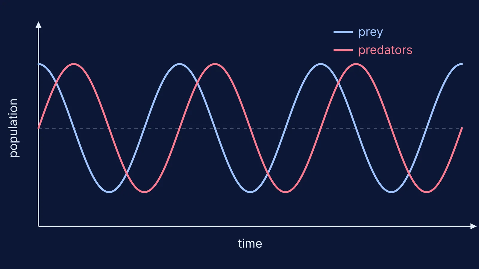
Follow one loop. Plenty of prey feeds the predators, so they multiply. More predators eat more prey, so prey fall. With food scarce, predators starve. With fewer hunters, prey bounce back, and the loop restarts.
The key detail is the lag: predators keep multiplying as long as prey stay above their balance level, so predators peak only after prey have started to fall. Near the balance point, the Wikipedia summary explains, the equations behave like simple harmonic motion, with predators trailing prey by 90°, a quarter of a cycle. The diagram above shows this lag.
The equations also have a conserved quantity, so each starting point traces its own closed loop instead of spiralling inward or outward.
A worked example you can do on paper
These numbers are made up for practice.
Choose α = 1, β = 0.1, γ = 1.5 and δ = 0.075.
Find the balance point. Set dy/dt = 0: δx = γ, so x* = 1.5 ÷ 0.075 = 20 prey.
Set dx/dt = 0: βy = α, so y* = 1 ÷ 0.1 = 10 predators.
Test a point. At x = 30, y = 10, dx/dt = 30 − 30 = 0 and dy/dt = −15 + 22.5 = +7.5. Prey are steady for a moment, but predators are rising: the loop is turning.
Now add fishing that removes a fraction f = 0.5 of both species each unit of time. Prey growth becomes α − f = 0.5 and predator death becomes γ + f = 2. The new balance is x* = 2 ÷ 0.075 ≈ 26.7 prey and y* = 0.5 ÷ 0.1 = 5 predators.
Fishing lowers the predators' balance point and raises the prey's. Run it backwards and you get D'Ancona's puzzle: stop fishing, as the war did, and the predator share goes up.
If these curves are hard to picture from algebra, the Fermi Simulation Lab has interactive simulations for ideas that are easier to see than to read. You can also sketch them by hand with slope fields.
Does the model match real animals?
Sometimes, roughly. Hudson's Bay Company fur records of lynx and snowshoe hare rise and fall repeatedly, and Charles Elton and Mary Nicholson described "The Ten-Year Cycle in Numbers of the Lynx in Canada" in The Journal of Animal Ecology in 1942.
The simple model leaves out food limits for prey, predators switching prey, and weather. Its lasting lesson is that two linked feedback loops can make a cycle with no outside push. For another case of simple equations shaping living things, read how Alan Turing's maths explained animal coat patterns.
If a term in the equations still feels shaky, the Fermi Concept Library gives each concept in biology and mathematics its own lesson, so you can fill the gap before your next problem set.