

On this page
A slope field turns a differential equation into a picture before you solve anything. Read the picture and you can predict the answer's shape, catch sign errors, and see why hot chai never cools below room temperature.
What is a slope field in a differential equation?
A direction field, also called a slope field, is "a mathematical object used to graphically represent solutions to a first-order differential equation", says the OpenStax Calculus Volume 2 chapter on direction fields. At each point you draw a short segment whose slope is the value of dy/dx the equation gives there. A solution curve runs along those segments, touching each like a tangent.
The same chapter defines an equilibrium solution as a constant solution y = c, found by setting the right-hand side to zero. Nearby curves either settle towards these flat lines (stable) or move away from them (unstable).
How do you draw a slope field by hand?
Use this four-step routine for dy/dx = f(x, y).
Find the equilibria: set f = 0 and draw those horizontal lines first.
Mark the signs: above and below each equilibrium, are slopes positive (rising) or negative (falling)?
Compute a few slopes. When f depends only on y, every point on a horizontal line has the same slope, so one calculation fills a row.
Draw short segments, steeper where f is larger in size. Then put your pencil on the starting point and follow them.
How do growth, decay and cooling look in a slope field?
Predict first, then check against the solution.
Growth, dy/dt = 0.5y. Equilibrium: y = 0. Above it the slope doubles when y doubles: 0.5 at y = 1, 1 at y = 2, 2 at y = 4. Prediction through (0, 1): a curve that starts gently and bends ever more steeply upwards. Check: y = e^(0.5t), so y is about 2.72 at t = 2 and doubles every ln 2 / 0.5, about 1.39 time units. Curves near y = 0 move away from it: unstable.
Decay, dN/dt = -0.2N. Equilibrium: N = 0. Through (0, 100) the first slope is -20; at N = 50 it is only -10. Prediction: a fast fall that flattens towards the axis without touching it. Check: N = 100e^(-0.2t), half-life ln 2 / 0.2, about 3.47 time units. This is radioactive decay's shape; see our post on solving growth and decay differential equations.
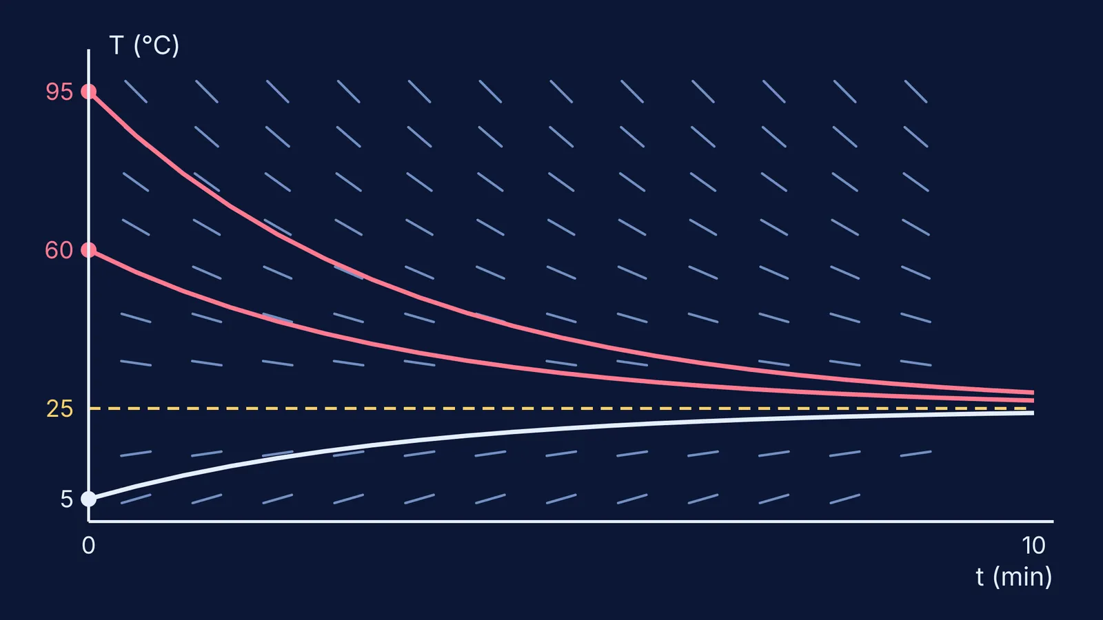
Cooling, dT/dt = -0.3(T - 25). T is temperature in °C, t is time in minutes and the room is at 25 °C. Equilibrium: T = 25. Slopes are negative above it and positive below, so curves from both sides head towards 25: stable. Chai at 95 °C starts falling at 0.3 × 70 = 21 °C per minute; at 60 °C the rate has halved to 10.5. Water from the fridge at 5 °C starts warming at 6 °C per minute.
Prediction: a steep fall, then a flattening approach to 25 °C from above, while the cold water climbs to meet it from below. Check: T = 25 + 70e^(-0.3t) gives about 40.6 °C after 5 minutes. The physics behind this model is in our explainer on Newton's law of cooling.
How do you predict the solution curve through a point?
Follow the segments in small steps. From (0, 95) on the cooling field, a one-minute step along the starting slope of -21 lands at 74 °C. The exact value at t = 1 is 25 + 70e^(-0.3), about 76.9 °C. The straight step undershoots because the curve bends upwards as the slope gets gentler. This tracing is Euler's method, which the OpenStax chapter covers next; smaller steps shrink the error.
Before you integrate, answer three questions:
Where does the curve go as t grows: to an equilibrium, or off to infinity?
Is it rising or falling at the start, and roughly how fast?
Does it bend upwards or downwards?
If your algebra disagrees with any answer, recheck the algebra. If you cannot find the slip, the Fermi Problem Library has worked problems with a step-by-step solver that explains the reasoning rather than printing an answer.
Does sketching first help you understand differential equations?
There is some classroom evidence. Diarmaid Hyland, Paul van Kampen and Brien Nolan taught direction fields in a fifty-minute guided-inquiry tutorial, one of fifteen in an ODE module for physics undergraduates and prospective maths teachers at an Irish university (International Journal of Mathematical Education in Science and Technology, 2019; author manuscript). They report that a large majority of students who completed the tutorial could do tasks linking direction fields to ODEs, and that over the whole intervention students' ideas of what a solution is improved significantly. One study is not a guarantee, but it suggests direction fields are worth learning.
Some ideas are easier to see than to read, and the Fermi Simulation Lab has interactive simulations for those. For plotting tools, see our guide to graphing tools for maths.
Tonight, pick one equation from your textbook, sketch its field, predict the curve through one point, and only then solve it.


