
On this page
Push a heavy almirah that will not budge, push harder, and it suddenly lurches forward. That moment is the whole story of the friction vs applied force graph, a Class 11 favourite. Once you can read its three parts, the rise, the peak and the drop, most friction questions become a single comparison.
What does the graph of friction force vs applied force look like?
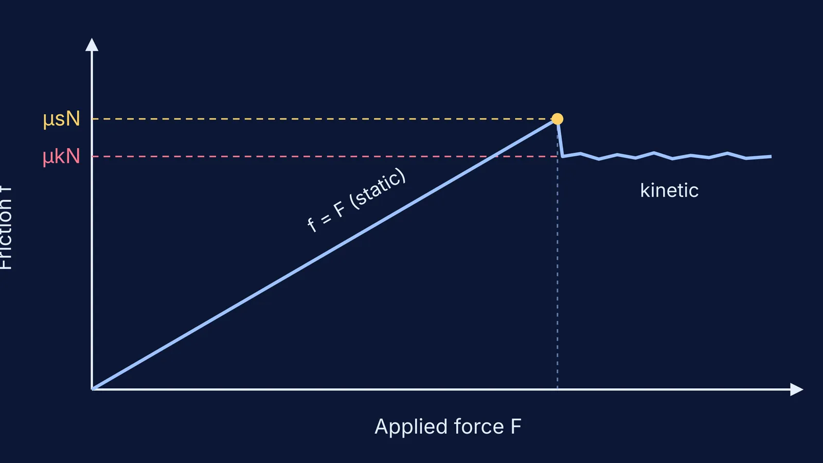
The standard picture in OpenStax University Physics, Volume 1, section 6.2 has three parts, with the applied force F on the horizontal axis and the friction force f on the vertical axis:
The static region. Friction equals the applied force, so the graph is a straight line through the origin with slope 1 (f = F).
The peak. The line stops at the maximum static friction, fs(max) = μsN, often called limiting friction. Once the applied force exceeds it, the object moves.
The kinetic region. Friction drops a little and then flattens out to a value that is noisy but constant on average, fk = μkN.
Static friction obeys fs ≤ μsN, while kinetic friction is fk = μkN, where N is the normal force (OpenStax, section 6.2).
Why does static friction rise with the applied force?
Static friction is self-adjusting. It is not a fixed number; it is whatever force is needed to stop the surfaces sliding, up to a limit. Push gently and friction pushes back just as hard; push harder and it matches that too, so the net force stays zero and the block stays at rest.
This is why μsN is a ceiling, not the answer. The most common mistake on this graph is to write f = μsN for a block that is not moving. To see how this force fits with energy, read our post on whether static friction can ever do work.
Why does friction drop once the block starts moving?
Once the push exceeds μsN, the block breaks free and friction becomes kinetic. OpenStax notes that kinetic coefficients are less than their static counterparts, so μs > μk and the graph has to step down (OpenStax, section 6.2).
The same textbook gives approximate values in its Table 6.1 (OpenStax):
Wood on wood: μs = 0.5, μk = 0.3
Steel on steel (dry): μs = 0.6, μk = 0.3
Rubber on dry concrete: μs = 1.0, μk = 0.7
Ice on ice: μs = 0.1, μk = 0.03
In every row the kinetic value is the smaller one. That gap is the drop on your graph, and it is why a box is easier to keep moving than to start. For how static, sliding and rolling friction rank against each other, read why static, sliding and rolling friction come in that order.
Worked example: what happens as you push a 20 kg crate harder?
This uses Example 6.10 from OpenStax University Physics, section 6.2: a 20.0 kg crate on a floor with μs = 0.700 and μk = 0.600. The hero graph above is drawn from these numbers.
Normal force: N = mg = 20.0 × 9.80 = 196 N.
Limiting friction: μsN = 0.700 × 196 = 137 N. This is the peak of the graph.
Push with 20.0 N, 30.0 N or 120.0 N: each is below 137 N, so the crate stays put and friction equals the push. These points sit on the f = F line.
Push with 180.0 N: this is more than 137 N, so the crate moves. Friction is now kinetic, μkN = 0.600 × 196 = 118 N.
Acceleration: a = (180.0 − 118) ÷ 20.0 = 3.10 m/s², as OpenStax finds.
Notice that friction never reads 180 N. In this model, once the crate slides, friction stays at 118 N whatever you push with, which is the flat part of the graph.
How do you answer a friction graph question in an exam?
Run this checklist on every friction problem, graph or not:
Find N first. On a flat floor with a horizontal push, N = mg; with an angled push or an incline, it changes.
Work out the limit μsN.
Compare: is the applied force below, equal to or above the limit?
Below: the block is at rest and f = F. Above: it slides, f = μkN, and you use F − μkN = ma.
Sketch the peak at μsN and the flat line below it at μkN.
If you keep picking μsN when the block is at rest, the gap is usually in the idea of a self-adjusting force rather than in the algebra. The Fermi Concept Library has each idea in physics with its own lesson, so you can go back to static and kinetic friction on their own. To practise the comparison step, the Fermi Problem Library has worked problems with a step-by-step solver that explains the reasoning rather than printing an answer.