
On this page
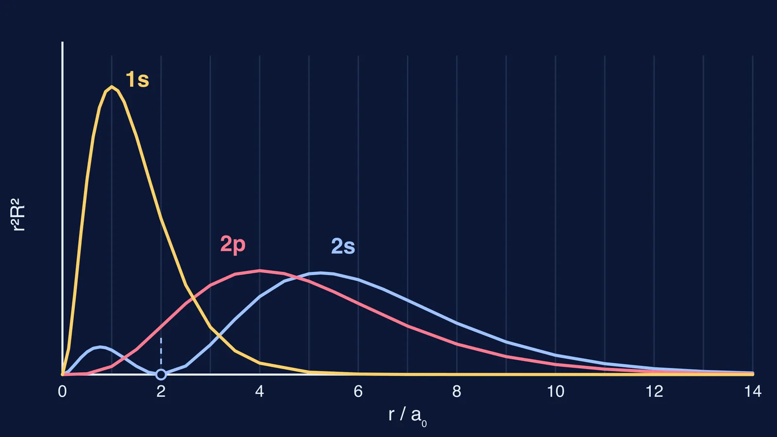
If you have stared at the textbook graph of radial probability against r and wondered why the 1s curve starts at zero when the electron is supposedly most likely to be at the nucleus, you are not alone. Both statements are true; they answer different questions. Here are the three hydrogen curves, where every peak and node comes from, and the equations to plot them yourself.
What does the radial probability distribution actually measure?
Picture the atom as an onion made of thin spherical shells. The radial probability is the chance of finding the electron in the shell at distance r, found by adding up the probability at every point on that shell (LibreTexts, Probability Density and Nodes). In symbols it is P(r) = r²R², where R is the normalised radial wavefunction (Wikiversity, The hydrogen atom). For an s orbital, ψ = R/√(4π), so the same quantity is often written 4πr²ψ².
Two things compete. For 1s, the probability density ψ² is greatest at the nucleus, but a shell that close has so little surface area that the total probability there vanishes (LibreTexts, The Shape of Atomic Orbitals). Far out, the shells are huge but ψ² has died away. Multiply a growing r² by a shrinking R² and you get a hump.
Where are the peaks of the 1s, 2s and 2p curves?
Measure r in Bohr radii. The Bohr radius a₀ is 5.29177 × 10⁻¹¹ m, about 52.9 pm (NIST CODATA value). The standard hydrogen radial functions are R(1s) ∝ e^(−r/a₀), R(2s) ∝ (2 − r/a₀)e^(−r/2a₀) and R(2p) ∝ (r/a₀)e^(−r/2a₀) (Wikiversity). Writing x = r/a₀ and normalising so each curve has total area 1:
1s: P = 4x²e^(−2x)
2s: P = x²(2 − x)²e^(−x) / 8
2p: P = x⁴e^(−x) / 24
Now find each peak by setting dP/dx = 0.
1s. dP/dx is proportional to x(1 − x)e^(−2x), which is zero at x = 1. The peak sits at one Bohr radius, 52.9 pm, the same radius Bohr calculated for the n = 1 orbit (LibreTexts).
2p. dP/dx is proportional to x³(4 − x)e^(−x), so the peak is at x = 4, about 212 pm.
2s. Let f = x(2 − x). Then dP/dx is proportional to f(x² − 6x + 4)e^(−x). It vanishes at x = 2 (the node) and at x = 3 ± √5. That gives a small inner hump at 0.76a₀ (about 40 pm) and the main hump at 5.24a₀ (about 277 pm).
So the 2s main peak lies farther out than the 2p peak, yet 2s also has an inner hump where the 2p curve is almost flat: at 0.76a₀ the 2s curve is about eight times higher. Integrate the 2s curve from 0 to 2a₀ and about 5% of its probability sits inside the node.
How do you count radial nodes with n − l − 1?
The number of radial nodes is n − l − 1 (LibreTexts). Angular nodes equal l, and the total is n − 1 (LibreTexts, Radial Nodes/Quantum_Mechanics/09._The_Hydrogen_Atom/Radial_Nodes)). Check it against the curves:
1s: 1 − 0 − 1 = 0 radial nodes, one hump.
2s: 2 − 0 − 1 = 1 radial node, at r = 2a₀, where the factor (2 − r/a₀) becomes zero (Wikiversity). Two humps.
2p: 2 − 1 − 1 = 0 radial nodes, one hump. Its single node is angular, a nodal plane through the nucleus.
3s: 3 − 0 − 1 = 2 radial nodes, three humps.
Self-check: a curve has one more hump than it has radial nodes, so n − l humps in all.
For more practice, see counting radial and angular nodes for any orbital; for the shapes behind these curves, see atomic orbitals visualised in 3D.
How can you plot these curves yourself?
An interactive graph lets you test predictions. Open any free graphing calculator and try this 15-minute plan.
Type the three equations above with x from 0 to 15. Colour them differently.
Before zooming, write down where you expect the 2s node. Then zoom in and check that the curve touches zero at x = 2.
Click each maximum. You should read 1, 0.76, 5.24 and 4.
Shade the area under the 2s curve from 0 to 2. It should come to about 0.05.
Predict how many humps a 3s curve should have before you look one up.
If the counting of n, l and subshells is still shaky, our explainer on how many subshells and orbitals each shell holds is a good warm-up. And if you would rather drag a slider than type equations, the Fermi Simulation Lab has interactive simulations for ideas that are easier to see than to read.
Plot the 2s curve once, find its node with your own eyes, and n − l − 1 stops being a formula you memorise.