
On this page
A tree diagram turns a confusing "given that" question into arithmetic you can see. Below we build one for drawing balls without replacement, vary the ball counts like sliders, and check the answer by simulation, so you trust the formula because you watched it work.
We use the urn from Example 8 in the NCERT Class 12 probability chapter: 10 black balls and 5 white balls, two drawn one after the other without replacement.
How do you draw a tree diagram for drawing without replacement?
NCERT defines conditional probability as P(E|F) = P(E ∩ F) / P(F), provided P(F) is not zero (NCERT, section 13.2). Rearranged, this is the multiplication rule, P(E ∩ F) = P(E) P(F|E), which is exactly what a tree does along each path.
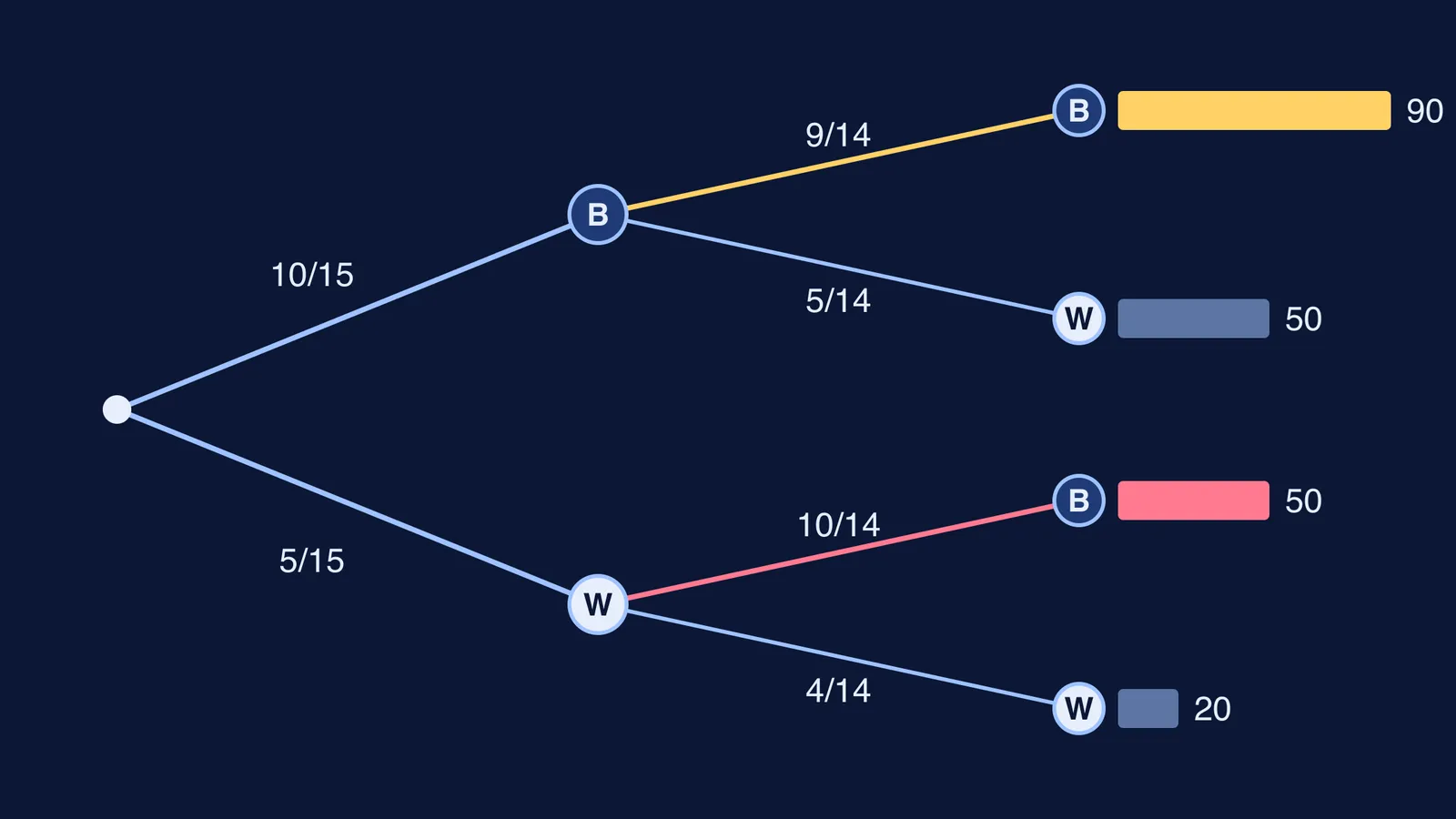
Draw two branches for the first ball: black with 10/15, white with 5/15.
From the black node, the urn now holds 9 black and 5 white, so the branches are 9/14 and 5/14.
From the white node, it holds 10 black and 4 white, so the branches are 10/14 and 4/14.
Multiply along each path. Black-black is 10/15 × 9/14 = 90/210, which NCERT simplifies to 3/7. Black-white and white-black are each 50/210. White-white is 20/210.
Check that the four ends add to 210/210.
"Without replacement" lives only in the second column: denominators drop from 15 to 14, and the colour you drew loses a ball.
What is P(first black given second black)?
This question trips people up because it runs backwards in time.
Event B, "second ball is black", happens on two paths: black-black (90) and white-black (50). That is 140 out of 210, or 2/3.
Event A and B together, "both black", is the single path of 90.
So P(first black | second black) = 90/140 = 9/14, about 0.643.
Notice two things. First, P(second black) is 2/3, the same as P(first black) = 10/15: before you look, the second draw is no more likely to be black. Second, learning that the second ball is black lowers the chance for the first from 10/15 to 9/14, because one black ball is already accounted for.
Gerd Gigerenzer and Ulrich Hoffrage found that when Bayesian problems were presented in frequency formats rather than probabilities, statistically naive participants derived up to 50% of their inferences by Bayesian algorithms, without instruction (Psychological Review, 1995). The 90-and-50 counts above are a frequency format.
If you want the same idea with two dice, see our walk-through of conditional probability as a reduced sample space.
What happens when you change the counts with sliders?
Replace 10 and 5 with b black and w white. The tree gives black-black = b(b−1) and white-black = wb, so P(first black | second black) = (b−1)/(b−1+w). Make b and w two slider cells in a spreadsheet, or use a pencil, and predict before computing:
b = 1: the answer is 0. If the only black ball came second, the first cannot be black.
w = 0: the answer is 1. Every ball is black.
b = 2, w = 5: the answer drops to 1/6.
b = 100, w = 50: the answer is 99/149, about 0.664, very close to 2/3.
The last case shows when replacement stops mattering: with replacement the draws are independent and the answer is always b/(b+w), and in a big urn removing one ball barely changes it.
How do you check P(A given B) by simulation?
A simulation tests the same NCERT urn (chapter PDF) without any formula. You can run it with 15 paper chits in a box or a few lines of code.
Shuffle 10 black and 5 white, then take the first two.
Repeat many times, say 10,000.
Throw away every run where the second ball is white. About two-thirds of runs, roughly 6,667, survive.
Among the survivors, find the fraction where the first ball is black.
That fraction should sit near 0.643. With about 6,667 survivors the standard error is about 0.006, so most repeats of the experiment land between 0.63 and 0.66. Step 3 is the definition of conditioning: you shrink the world to the cases where B happened, then count A inside it.
Why the estimate settles as runs pile up is the subject of our post on 10,000 coin tosses and the law of large numbers. For a famous puzzle where simulation beats intuition, try the two child problem simulation.
For more ideas that are easier to see than to read, the Fermi Simulation Lab has interactive simulations you can explore. If a conditional probability question still goes wrong at the method stage, the Fermi Problem Library has worked problems with a step-by-step solver that explains the reasoning rather than printing an answer.
Next time you see "given that", draw the tree, count the paths where the condition holds, and run the chits once to check.