
On this page
A square wave flips between +1 and −1, with flat tops and vertical edges, like the clock signal in a digital circuit. A sine wave is smooth everywhere. Yet you can build the square from sines alone. Here is the recipe, a worksheet to plot by hand, and the one flaw that never goes away.
Which sine waves add up to a square wave?
A square wave of height 1 equals (4/π)[sin t + (1/3) sin 3t + (1/5) sin 5t + (1/7) sin 7t + …], a sum of odd harmonics only (Wikipedia: Square wave)). Wolfram MathWorld gives the same series, with each term's amplitude proportional to 1/n (MathWorld: Fourier series of a square wave).
So the recipe has three rules:
Use only odd multiples of the base frequency: 1, 3, 5, 7 and so on.
Shrink each in proportion: the third harmonic is one third as tall, the fifth one fifth.
Start them together, all crossing zero upwards at t = 0.
Why only odd ones? The second half of a square wave is the first half turned upside down. An odd harmonic such as sin 3t also flips sign after half a period, so it fits; an even one such as sin 2t does not.
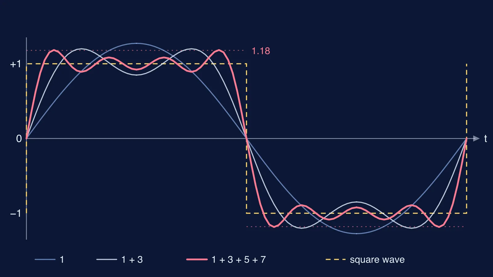
What happens when you add harmonics 1, 3, 5 and 7?
We worked out the running total from the series above at t = 0°, 15°, 30°, 45°, 60°, 75° and 90°. Each row adds one harmonic.
1 only: 0, 0.330, 0.637, 0.900, 1.103, 1.230, 1.273
1 + 3: 0, 0.630, 1.061, 1.200, 1.103, 0.930, 0.849
1 + 3 + 5: 0, 0.876, 1.188, 1.020, 0.882, 0.996, 1.103
1 + 3 + 5 + 7: 0, 1.051, 1.097, 0.892, 1.040, 1.043, 0.922
How do you plot the sums by hand?
Draw a t axis from 0° to 360°, ticks every 15°, and a y axis from −1.3 to +1.3. Dashed lines at +1 and −1 are your target.
Plot the first row from 0° to 90°. Mirror it for 90° to 180°: the value at 180° − t equals the value at t.
For 180° to 360°, each value is minus the value 180° earlier.
Before each new row, predict where the curve will rise and dip. Then plot it in a new colour.
Check one number in degree mode: 1 + 3 at 45° is (4/π)(0.7071 + 0.7071/3) = 1.200.
Three patterns appear. The edges get steeper: at 15° the sum climbs from 0.330 to 1.051 as you go from one term to four. The top gets flatter but ripplier: N terms make N humps between 0° and 180°. And the tallest hump slides towards the jump. The slope of the sum of the first N odd terms is (2/π) sin(2Nt)/sin t, which first hits zero at t = 90°/N. So the peak sits at 90°, 45°, 30° and then 22.5° as you add harmonics 1, 3, 5 and 7.
Why does the overshoot never go away?
Now read off the peak heights: 1.273, 1.200, 1.188 and 1.184 (the last at 22.5°). They fall, but not to 1. The overshoot next to a jump settles at about 9% of the jump, and the overshoot peaks only move closer to the jump as more terms are summed (Wikipedia: Gibbs phenomenon). Here the jump is 2, from −1 to +1, so the peaks approach about 1.179 however many harmonics you add. The overshoot gets thinner while staying just as tall, so the area of the error heads to zero: pointwise convergence that is not uniform, in the same article's words.
That article also records that Henry Wilbraham noticed the effect in 1848 and that Maxime Bôcher named it the Gibbs phenomenon in 1906. J. Willard Gibbs wrote about it in letters to Nature in 1898 and 1899; the second, “Fourier's Series”, appeared on 27 April 1899 (Nature, doi:10.1038/059606a0). Edwin and Robert Hewitt retold the story in 1979 as “The Gibbs-Wilbraham phenomenon” (Archive for History of Exact Sciences). The ringing at the edges of real square waves is also related to it (Wikipedia: Square wave)).
How can you watch the harmonics add up?
Your hand plot gives four snapshots; a slider for the number of terms would show the ripples crowding the edge. Ideas that are easier to see than to read are what the interactive simulations in the Fermi Simulation Lab are for. If harmonics or superposition feel shaky, the Fermi Concept Library has a lesson for each concept in physics and mathematics.
The same odd-and-even thinking explains which harmonics go missing when you pluck a string at L/3. For two waves of the same frequency, see adding two SHMs with the phasor method, and for waves at right angles, predicting Lissajous figures before you simulate.
One last test once your four rows are plotted: add (1/9) sin 9t and check that the peak lands at 18°, at about 1.182.