
On this page
William George Horner was a schoolmaster, not a university professor. According to the MacTutor biography, he was born in Bristol in 1786, became headmaster of Kingswood School in 1804, and in 1809 founded his own school in Bath, where he died in 1837. His name is now attached to the steps you use in synthetic division.
What is Horner's method?
Horner's method evaluates a polynomial by nesting it: a3x³ + a2x² + a1x + a0 becomes ((a3x + a2)x + a1)x + a0. You start with the leading coefficient, multiply by x, add the next coefficient, and repeat.
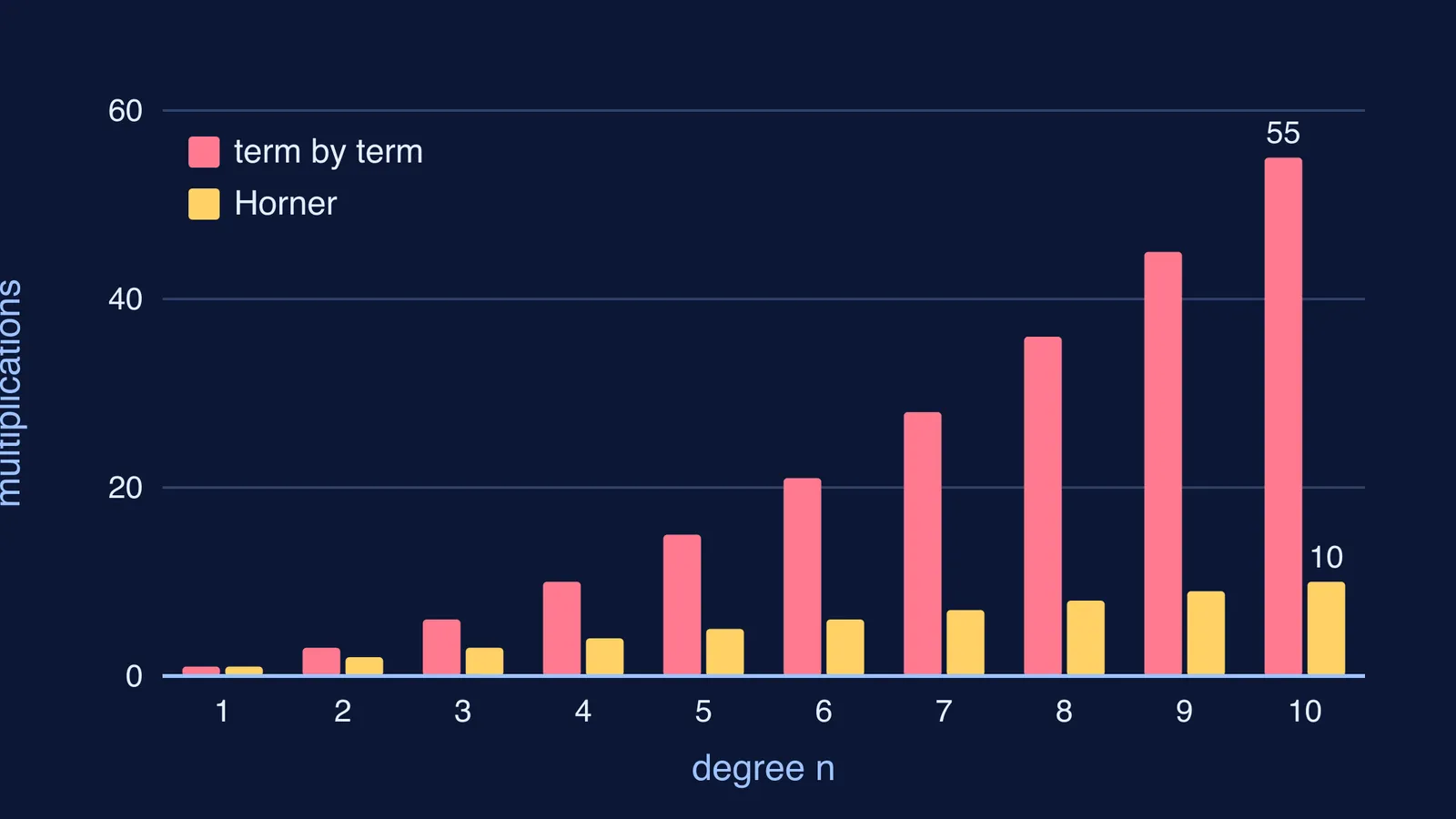
For a polynomial of degree n, Horner's method needs only n multiplications and n additions, as the summary of the method on Wikipedia sets out. Working term by term, where you build each power of x from scratch, costs (n² + n)/2 multiplications. For a degree-10 polynomial that is 55 multiplications against 10.
For a general polynomial, with no preprocessing of the coefficients, you cannot do better. The same Wikipedia article records that Alexander Ostrowski proved in 1954 that the number of additions is minimal, and Victor Pan proved in 1966 that the number of multiplications is minimal (Pan, Russian Mathematical Surveys, 1966).
How do you evaluate a polynomial with Horner's method?
Take p(x) = 2x³ − 6x² + 2x − 1 and find p(3). Write the coefficients in order: 2, −6, 2, −1. Never skip a power; a missing term gets a 0.
Bring down the first coefficient: 2.
Multiply by 3 and add the next coefficient: 2 × 3 = 6, then 6 + (−6) = 0.
Again: 0 × 3 = 0, then 0 + 2 = 2.
Again: 2 × 3 = 6, then 6 + (−1) = 5.
So p(3) = 5. Check it the long way: 54 − 54 + 6 − 1 = 5. Term by term you needed six multiplications (three for 2·3·3·3, two for 6·3·3, one for 2·3). Horner needed three.
How did Horner use it to solve equations?
Horner's 1819 paper, "A new method of solving numerical equations of all orders, by continuous approximation", appeared in the Philosophical Transactions of the Royal Society. The root-finding procedure later taught under his name finds a root one digit at a time. Here is the idea, applied to x³ − 2x − 5 = 0.
Find the whole-number part. p(2) = −1 and p(3) = 16, so the root lies between 2 and 3.
Shift the equation. Put x = 2 + y. Running the Horner row with 2 again and again gives the new coefficients: y³ + 6y² + 10y − 1 = 0.
Find the next digit. y is small, so 10y ≈ 1 suggests y ≈ 0.1. Testing shows the value at 0.1 is just above zero and at 0.09 just below, so the digit is 9 and x ≈ 2.09.
Shift again by 0.09 and repeat. Each round adds a digit; the root is about 2.0946. Only multiplication and addition, which suited hand calculation.
Did Horner really invent Horner's method?
No. The Wikipedia history of the method records that Qin Jiushao's Mathematical Treatise in Nine Sections (1247) presents Horner-type methods for solving polynomial equations. The MacTutor biography notes that Zhu Shijie had considered it in China centuries earlier and that Paolo Ruffini anticipated it in Europe; you can read more in our posts on Qin Jiushao and the remainder theorem and on Ruffini and synthetic division.
Even the English credit is disputed. In 1999 A. Thomas Fuller argued in Historia Mathematica that the method in Horner's 1819 paper differs from what later became known as Horner's method, and that priority should go to Theophilus Holdred, who published it in 1820. MacTutor adds that Augustus De Morgan gave Horner's name and method wide coverage in many articles.
When should you use Horner's method in an exam?
In school algebra it appears as synthetic division. Use it when you:
need p(a) for a polynomial of degree 3 or more
test trial roots for the factor theorem, where you want p(a) = 0
divide by (x − a) and need both quotient and remainder
Three habits help you avoid the usual slips:
Write a 0 for every missing power before you start.
Use a, not −a, when dividing by (x − a). For (x + 2), use −2.
Check the last number by substituting a once, the long way.
Our step-by-step guide to synthetic division of polynomials has more practice. If you keep dropping a zero or a sign, the Fermi Problem Library has worked problems with a step-by-step solver that explains the reasoning rather than printing an answer. To revisit the remainder and factor theorems themselves, the Fermi Concept Library gives each mathematics concept its own lesson.
Try it now: find p(−2) for x⁴ − 3x² + x + 7 with a Horner row, remembering the 0 for x³. You should get 9.