
On this page
Every biology and chemistry student meets the same curve. Add more substrate and an enzyme works faster, but the gains get smaller and the rate levels off. In 1934 two scientists at the US Department of Agriculture published a way to turn that curve into a straight line you can read with a ruler. Students still draw their graph more than 90 years later.
Who were Lineweaver and Burk?
The paper is "The Determination of Enzyme Dissociation Constants" by Hans Lineweaver and Dean Burk, in the Journal of the American Chemical Society, volume 56, pages 658–666, published in March 1934. The Crossref record lists more than 10,000 works that cite it.
Lineweaver was a graduate student working as a laboratory assistant under Burk at the USDA when he developed the equation, according to his biography. He earned a PhD at Johns Hopkins in 1936, spent 44 years at the USDA and died in 2009, aged 101.
Burk had joined the USDA's Fixed Nitrogen Research Laboratory in 1929. He moved to the National Cancer Institute in 1939 and worked with Otto Warburg on photosynthesis, according to his biography.
Did Lineweaver and Burk invent the double-reciprocal plot?
Not quite. Lineweaver's biography says Barnet Woolf had worked out this straight-line form and two others first. Injuries from a car accident kept him from publishing them, but J. B. S. Haldane mentioned them in a 1932 book on enzymes. The idea was largely ignored until Lineweaver and Burk found it again, and their names stuck. For this account the biography cites Haldane's 1957 note in Nature, "Graphical Methods in Enzyme Chemistry".
A second twist: according to the plot's reference entry, they consulted the statistician W. Edwards Deming and used weighted fitting, drawing the plot to show results rather than calculate them.
What problem did the double-reciprocal plot solve?
In 1913 Leonor Michaelis and Maud Menten published the work behind the rate law for enzymes; an English translation appeared in Biochemistry in 2011, and our post on Michaelis, Menten and the equation for enzyme speed tells their story. In textbook form the law reads v = Vmax[S] / (Km + [S]).
Vmax is the top speed, reached when every enzyme molecule is busy.
Km is the substrate concentration at which the rate is half of Vmax.
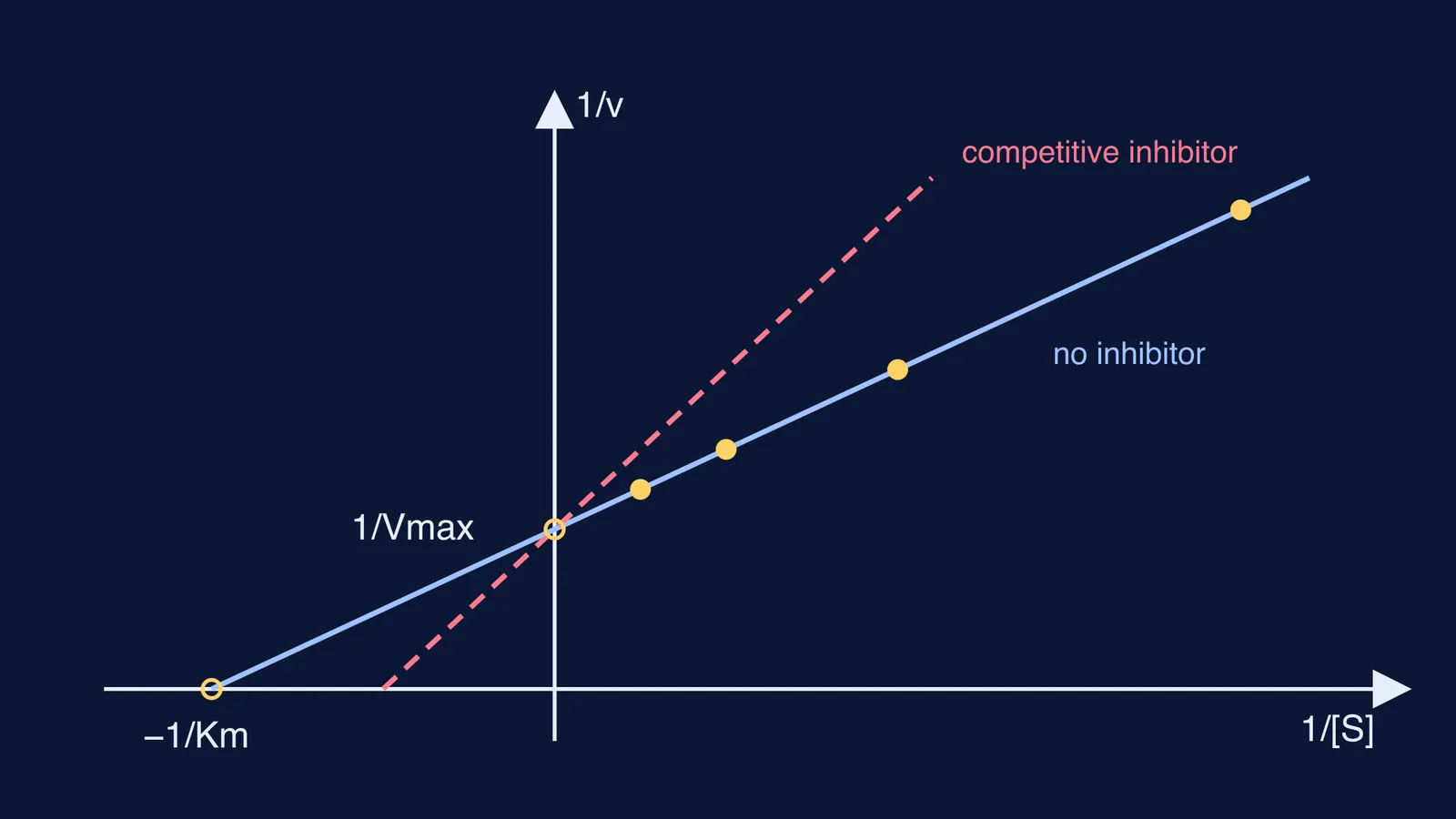
The curve only approaches Vmax and never reaches it, so guessing the plateau by eye is unreliable. Take the reciprocal of both sides and you get 1/v = (Km/Vmax)(1/[S]) + 1/Vmax, the form y = mx + c. The Lineweaver–Burk plot graphs 1/v against 1/[S]: the y-intercept is 1/Vmax, the slope is Km/Vmax and the x-intercept is −1/Km.
At high substrate the enzyme is saturated and the rate barely changes, much like a zero-order reaction; see zero and first order concentration-time graphs.
How do you find Km and Vmax from a Lineweaver–Burk plot?
Here is a worked example with made-up but self-consistent data for an enzyme with Km = 2 mM and Vmax = 10 µmol/min.
Measure the starting rate at four substrate levels: [S] = 1, 2, 4 and 8 mM give v = 3.33, 5.00, 6.67 and 8.00 µmol/min.
Take reciprocals: 1/[S] = 1, 0.5, 0.25, 0.125 and 1/v = 0.300, 0.200, 0.150, 0.125.
Plot them. The points fall on one line with slope 0.2 and y-intercept 0.1.
Vmax = 1/0.1 = 10 µmol/min.
Km = slope × Vmax = 0.2 × 10 = 2 mM. Check: the line crosses the x-axis at −0.5, and −1/Km = −0.5.
The most common slip is mixing up the intercepts. The y-axis is "infinite substrate" (1/[S] = 0), so that is where top speed lives.
Why do biochemists now distrust the plot?
Taking reciprocals stretches the errors. The plot's reference entry notes that it distorts the error structure of the data, and that properly weighted nonlinear regression is more accurate.
You can see why with the example above. Suppose every rate is measured to within ±0.5 µmol/min. At 8 mM, 1/v lands between 0.118 and 0.133, a spread of 0.015. At 1 mM, it lands between 0.261 and 0.353, a spread of 0.092, about six times wider. The least precise points sit furthest to the right and pull the line hardest.
Use the plot to read a graph quickly; let software fit the curve when the numbers matter.
How does a Lineweaver–Burk plot show an inhibitor?
Competitive inhibitor: same y-intercept, steeper line. Vmax is unchanged and Km goes up.
Pure non-competitive inhibitor: same x-intercept, higher y-intercept. Km is unchanged and Vmax goes down.
Uncompetitive inhibitor: a parallel line shifted up. Both Vmax and Km go down.
As the plot's reference entry notes, pure non-competitive inhibition is rare; mixed inhibition, which changes both intercepts, is more common.
If saturation, active sites or Km still feel loose, the Fermi Concept Library has a lesson for every concept in physics, chemistry, biology, mathematics and computing. For practice, the Fermi Problem Library has a step-by-step solver that explains the reasoning, so you can see which intercept you misread.