On this page
From 5 March 1950, five meteorologists spent 33 days and nights with ENIAC, one of the first electronic computers, and made the first weather forecasts computed by a machine (Lynch, 2008). They turned the physics of moving air into arithmetic a computer could repeat, step by step.
Who made the first computer weather forecast?
The work was published in 1950 by Jule Charney, Ragnar Fjørtoft and John von Neumann in the journal Tellus (Charney, Fjørtoft and von Neumann, 1950). The five who reached the machine at Aberdeen, Maryland, on 5 March 1950 were Charney, Fjørtoft, John Freeman, George Platzman and Joseph Smagorinsky, according to meteorologist Peter Lynch (Lynch, 2008).
Charney was born in California in 1917 and began graduate study at UCLA in mathematics before switching to meteorology around 1942 (IEEE Computer Society biography). He led the Princeton meteorology group from 1948 to 1956, then taught at MIT until his death in 1981. See also how the ENIAC programmers learned without a manual.
How did ENIAC turn physics equations into a forecast?
In his 1922 book, Lewis Fry Richardson described a forecast worked out by hand: the calculations took him more than six weeks to produce a six-hour forecast for one location (Met Office). His answer, a surface pressure change of 145 hPa in six hours, was wildly wrong because his starting pressure and wind data were out of balance, setting off large gravity-wave oscillations (Lynch).
Charney's fix was to simplify. His quasi-geostrophic equations kept the slow, large-scale motions that make weather and were free of the sensitivity to fast motions that had wrecked Richardson's result (IEEE Computer Society biography).
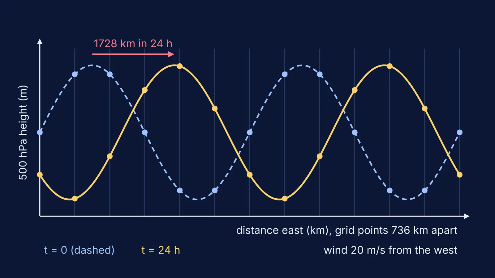
For ENIAC the team used the simplest version: the barotropic vorticity equation, which says that the absolute vorticity (spin) of a parcel of air stays constant as it moves (Lynch, 2008). Starting data came from the US Weather Bureau's hand-drawn 500 hPa map, read off on a grid of 19 by 16 points, 736 km apart at the North Pole.
ENIAC weighed 30 tons and held 18,000 vacuum tubes, but its internal memory was limited to about ten registers (Lynch, 2008). So each time step was split into 16 operations, with results punched onto cards and fed back in; about 100,000 cards were punched.
How good were the ENIAC forecasts?
The team made four 24-hour forecasts, all starting from weather maps from early 1949 (Lynch, 2008). Each 24-hour forecast took about 24 hours to compute. Lynch quotes Charney addressing the US National Academy of Sciences in 1955: "It mattered little that the twenty-four-hour prediction was twenty-four hours in the making. That was purely a technological problem."
In 2008 Lynch re-ran all four on a laptop. By root-mean-square error, simply assuming tomorrow's map equals today's (persistence) did better in three of four cases. By the S1 score, which measures how well the pattern of pressure gradients is predicted, all four forecasts showed some skill and three were clearly better than persistence.
By 1954 the US Weather Bureau, Air Force and Navy had set up a joint Numerical Weather Prediction Unit for routine daily forecasts (IEEE Computer Society biography). For how forecasting began a century earlier, read Robert FitzRoy and the first weather forecasts.
Can you do one forecast step by hand?
Yes, with a simpler cousin of ENIAC's equation: wind carrying a pattern of heights along unchanged. Rate of change of height = minus wind speed times height gradient. We use ENIAC's polar grid spacing, 736 km (Lynch, 2008).
Pick a grid point with 500 hPa height 5,580 m. The point 736 km to the west reads 5,520 m.
Gradient: (5,580 - 5,520) m / 736,000 m = 0.0000815.
Wind blows from the west at 20 m/s. Rate of change: -20 x 0.0000815 = -0.00163 m/s.
Step forward one hour (3,600 s): -0.00163 x 3,600 = -5.9 m.
New height: about 5,574 m, because lower heights are being carried in from the west.
Repeat that for every grid point, then for the next hour, and you have a forecast.
That stability rule is the CFL criterion. If picturing a wave sliding across a grid is the hard part, the Fermi Simulation Lab has interactive simulations for ideas that are easier to see than to read.
What can you learn from Charney's method?
The same habits work on a physics numerical:
Simplify first: keep the effect that matters and say what you dropped.
Check units at every line. Metres over metres, times metres per second, gives metres per second.
Compare with a simple baseline. The ENIAC forecasts were judged against "no change"; judge your answer against a rough estimate.
When you are wrong, name the cause. The 1950 paper tried to find the causes of its own errors.
Forecasts also have natural limits, part of the story of how Mary Cartwright and J.E. Littlewood found chaos.
To practise checking each step of a calculation, the Fermi Problem Library has worked problems with a step-by-step solver that explains the reasoning rather than printing an answer.