
On this page
Put a few yeast cells in a flask of sugar water and count them. At first little happens, then the numbers shoot up, then they stall. That S-shaped path is the logistic growth curve. NCERT Class 12 Biology, Chapter 11 (Organisms and Populations) sets it beside the exponential model and asks you to compare them.
What is the logistic growth equation?
NCERT writes logistic growth as dN/dt = rN(K − N)/K, where N is population density at time t, r is the intrinsic rate of natural increase and K is the carrying capacity (NCERT, Chapter 11).
Carrying capacity is the maximum population size that a particular environment can support (OpenStax Biology 2e, section 45.3).
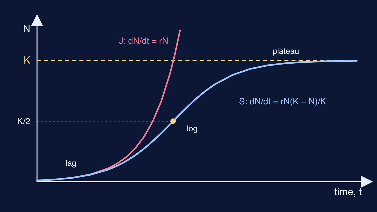
The exponential model is the same equation without the bracket: dN/dt = rN, which gives a J-shaped curve when you plot N against time (NCERT, Chapter 11). So the whole difference sits in (K − N)/K. Read it as "the fraction of room still left". When N is tiny, it is close to 1 and the population grows almost exponentially. When N reaches K, it becomes 0 and growth stops.
NCERT calls this Verhulst-Pearl logistic growth. Raymond Pearl and Lowell Reed published a mathematical representation of United States population growth since 1790 in PNAS in 1920. Our post on Pierre Verhulst and the logistic curve tells the earlier half of the story.
What are the phases of the logistic growth curve?
NCERT says a population in a habitat with limited resources shows a lag phase, then acceleration and deceleration, and finally an asymptote when it reaches the carrying capacity (NCERT, Chapter 11). You will also see the shorter labels lag, log and plateau. In equation terms:
Lag: N is small, so rN is small. The curve looks flat even though each individual is reproducing at nearly the full rate r.
Log or acceleration: N has grown, so rN is large and the bracket is still near 1. The curve bends upward steeply.
Deceleration: past K/2 the shrinking bracket outweighs the growing N, so each step adds fewer individuals.
Plateau or asymptote: N approaches K, the bracket approaches 0, and the curve flattens along the dashed K line.
How fast does a logistic population grow? A worked example
Take r = 0.12, the value NCERT quotes for the flour beetle (NCERT, Chapter 11), and an imagined habitat with K = 1,000. Compare the two models at three sizes:
N = 100: exponential gives 0.12 × 100 = 12; logistic gives 12 × 0.9 = 10.8.
N = 500: exponential gives 60; logistic gives 60 × 0.5 = 30.
N = 900: exponential gives 108; logistic gives 108 × 0.1 = 10.8.
Growth is fastest at N = K/2, where it equals rK/4 = 30; that is the steepest point of the S. The rates at 100 and 900 are equal, because rN(K − N)/K gives the same value at N and at K − N. And at N = 900 the two models differ tenfold.
With calculus, the solution is N(t) = K / (1 + ((K − N₀)/N₀)e^(−rt)). Starting from N₀ = 10, the population reaches K/2 at t = ln(99)/0.12, about 38 time units. At that moment the exponential model predicts 10 × 99 = 990, nearly double. The graph at the top of this post plots these two curves.
Why is logistic growth more realistic than the J curve?
NCERT's answer is short: since resources for most animal populations are finite and become limiting sooner or later, the logistic model is considered the more realistic one (NCERT, Chapter 11). The same chapter's r values show how species differ: 0.015 for the Norway rat, 0.12 for the flour beetle, and 0.0205 for India's human population in 1981.
Yeast grown in a test tube follows the classic S-shaped curve (OpenStax, section 45.3). Wild populations are messier: the same OpenStax section describes sheep and harbor seals whose numbers exceed the carrying capacity for short periods and then fall below it. So the logistic curve is a better model, not a perfect one.
How should you revise logistic growth for exams?
Before a board or NEET-UG test:
Draw both curves on one pair of axes, with K as a dashed line and K/2 marked.
Write both equations and say what the bracket equals at N = 0, K/2 and K.
Label the four NCERT phases on your S curve.
Redo the worked example with a new K, say 400, and check the peak rate is rK/4.
To see the curves move as you change r and K, try our population growth simulation post, and for the rest of the chapter read organisms and populations: growth models and species interactions.
If the bracket still feels slippery, the Fermi Concept Library has a lesson for every concept in biology and mathematics, each with its place in the map, and the Fermi Simulation Lab has interactive simulations for ideas that are easier to see than to read.