
On this page
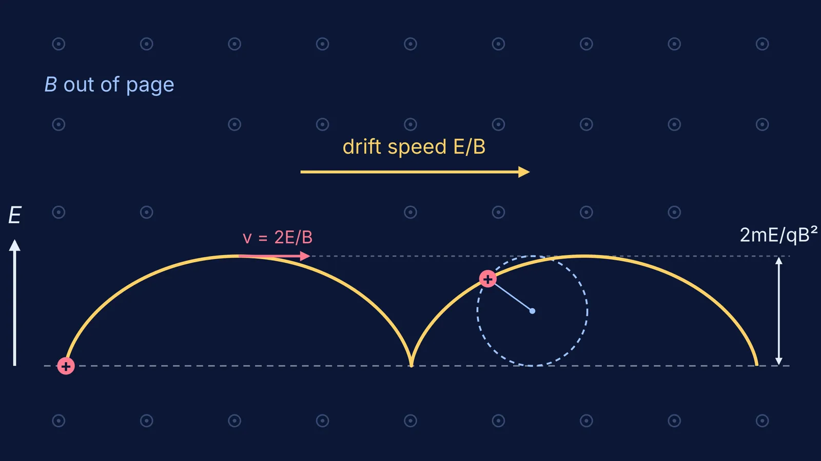
Put a uniform electric field E along +y and a uniform magnetic field B out of the page (along +z), then release a positive charge q of mass m at the origin. It neither flies off along E nor loops in a closed circle. It traces a row of arches, like a pebble stuck in a rolling bicycle tyre: a cycloid.
Why does the charge trace a cycloid?
Start from the Lorentz force, F = q(E + v × B). With B along z and E along y, the components are m dv_x/dt = qB v_y and m dv_y/dt = qE − qB v_x, as set out in Jeremy Tatum's Electricity and Magnetism text on LibreTexts/08:_On_the_Electrodynamics_of_Moving_Bodies/8.04:_Charged_Particle_in_an_Electric_and_a_Magnetic_Field). Nothing acts along z, so the motion stays in the xy-plane.
The key step: split the x-velocity into a constant part and a leftover: v_x = E/B + u. Substitute, and the qE term cancels exactly:
m du/dt = qB v_y
m dv_y/dt = −qB u
These are the equations for a charge in a magnetic field alone, so (u, v_y) turns in a circle at the cyclotron angular speed ω = qB/m. In a frame sliding along x at E/B, the charge simply goes round a circle, and the lab sees that circle carried along at E/B.
At t = 0 the charge is at rest, so u = −E/B and v_y = 0. The speed around the circle is therefore E/B, and the radius is r = (E/B)/ω = mE/qB². The centre moves at E/B and the rim turns at E/B too. Equal speeds mean a wheel rolling without slipping, and a point on its rim traces a cycloid.
What is the drift speed, and why is it E/B?
The guiding centre drifts at V_D = E/B, the drift velocity named in the LibreTexts derivation/08:_On_the_Electrodynamics_of_Moving_Bodies/8.04:_Charged_Particle_in_an_Electric_and_a_Magnetic_Field). It is the one speed at which the magnetic force qvB exactly balances the electric force qE, which is why subtracting it removed qE. Notice that q and m drop out: a proton, an electron and an alpha particle all drift at E/B in the same direction, along E × B. Only the size of their loops differs, and a negative charge loops on the opposite side of the starting line.
The same balance, qE = qvB, is how a velocity selector uses crossed fields: a charge that enters already moving at E/B along E × B feels no net force and goes straight, so the cycloid shrinks to a line.
Where does the maximum displacement 2mE/qB² come from?
Solving with the charge starting from rest at the origin gives:
x = (E/B)t − r sin ωt
y = r(1 − cos ωt), with r = mE/qB²
These match the parametric equations in the LibreTexts text. y is largest when cos ωt = −1, at ωt = π, so the maximum displacement along E is y_max = 2r = 2mE/qB².
Now check with energy. The magnetic force does no work, so all the kinetic energy comes from the electric field: ½mv² = qEy. At the top, v_x = (E/B)(1 − cos ωt) = 2E/B and v_y = 0. Then ½m(2E/B)² = qE·y_max gives y_max = 2mE/qB² again. Two routes, one answer. Each arch takes T = 2πm/qB, and the cusps are 2πr apart.
Worked example: an electron released from rest
Take E = 1.0 × 10³ V/m and B = 1.0 × 10⁻² T. The electron's charge-to-mass ratio has magnitude 1.758 820 008 38 × 10¹¹ C/kg, according to the NIST CODATA value.
Drift speed: E/B = 10³ / 10⁻² = 1.0 × 10⁵ m/s, along E × B.
Angular speed: ω = (e/m)B = 1.76 × 10⁹ rad/s.
Radius: r = (E/B)/ω = 5.7 × 10⁻⁵ m.
Maximum displacement: 2r = 1.1 × 10⁻⁴ m, about 0.11 mm, on the side opposite E because the electron is negative.
Peak speed: 2E/B = 2.0 × 10⁵ m/s, far below the speed of light, so the non-relativistic equations hold.
Time per arch: 2π/ω = 3.6 × 10⁻⁹ s; cusps 2πr = 0.36 mm apart.
How do you solve crossed-field questions in an exam?
A checklist for any JEE-style crossed-field problem:
Fix axes: E along y, B along z. E × B gives the drift direction.
Read the starting velocity. From rest gives sharp cusps; exactly E/B along E × B gives a straight line; most other starts give loops or ripples.
Subtract the drift, solve the circle, add the drift back.
Find the turning point from energy, qEy = ½mv².
Check dimensions: mE/qB² must come out in metres.
If the rolling wheel is still hard to picture, the Fermi Simulation Lab has interactive simulations for ideas that are easier to see than to read. For practice, the Fermi Problem Library has worked problems with a step-by-step solver that explains the reasoning, so you can see where your own working went off track. For the three-dimensional cousin of this motion, read how a charge follows a helical path in a magnetic field.