On this page
Two sets of numbers can share the same mean and look nothing alike. Standard deviation tells them apart, and with practice you can estimate it from a dot plot before touching the formula.
What does standard deviation actually measure?
The NIST/SEMATECH e-Handbook of Statistical Methods describes variance as "roughly the arithmetic average of the squared distance from the mean". Standard deviation is the square root of the variance, which, the same handbook notes, "restores the units of the spread to the original data units".
So read standard deviation as the typical distance of a data point from the mean. If a class's marks have a standard deviation of 10, a typical student sits roughly 10 marks from the average.
Two consequences are easy to see in a picture:
Squaring makes far-away points count heavily. One point 40 away adds 1,600 to the sum of squares; four points 10 away add only 400 between them.
Sliding every value by the same amount moves the mean but not the distances, so the standard deviation stays put (more in how adding or multiplying by a constant changes mean and variance).
How do you see the spread of data in a dot plot?
The NCERT Class 11 mathematics chapter on statistics opens with two batsmen's last ten scores:
Batsman A: 30, 91, 0, 64, 42, 80, 30, 5, 117, 71
Batsman B: 53, 46, 48, 50, 53, 53, 58, 60, 57, 52
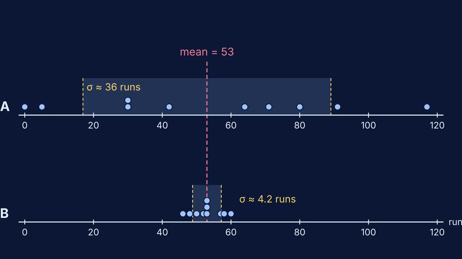
Both have a mean of 53 and a median of 53, the textbook points out, yet A's range is 117 and B's is 14. Plot them as dots on a number line, as NCERT does, and the difference is obvious: A's dots scatter from 0 to 117, B's bunch between 46 and 60. The image at the top of this post adds the mean line and shades one standard deviation either side.
Worked example: the two batsmen
Dividing by n = 10, as the NCERT chapter does (samples differ; see why variance divides by n in school and n − 1 in samples):
Mean: 530 ÷ 10 = 53 for both.
Deviations for A: −23, 38, −53, 11, −11, 27, −23, −48, 64, 18. They sum to zero, as deviations from the mean always do.
Sum of squares: 13,006 for A. B's deviations (0, −7, −5, −3, 0, 0, 5, 7, 4, −1) give 174.
Variance: 1,300.6 for A, 17.4 for B.
Standard deviation: about 36.1 runs for A, 4.2 runs for B.
Check it against the picture. A's scores sit 31.6 runs from the mean on average; B's sit 3.2. Each standard deviation is a little larger than that average distance because squaring gives extra weight to far dots like A's 0 and 117.
Which data set has the larger spread?
Sketch each pair as dots, commit to a prediction, then check.
P: 1, 2, 3, 4, 5 and Q: 101, 102, 103, 104, 105. Same spread: Q is P slid 100 to the right, so both standard deviations are √2, about 1.41.
R: 2, 4, 6, 8, 10 and S: 4, 8, 12, 16, 20. S is R stretched by 2, so its standard deviation doubles, from about 2.83 to 5.66.
C: 44, 44, 44, 44, 62, 62, 62, 62 and D: 35, 53, 53, 53, 53, 53, 53, 71. Both means are 53 and D's range (36) is double C's (18), so D looks more spread out. Yet both standard deviations are exactly 9. Every dot in C is 9 from the mean; in D, two dots are 18 away and six sit on it, and (2 × 18²) ÷ 8 = 81. Range sees only the end dots; standard deviation counts every dot.
The rules behind those answers:
Dots further from the mean line: larger standard deviation.
Sliding the whole plot: no change.
Multiplying every value by a positive number k: standard deviation times k.
A few distant dots can outweigh many close ones.
Why does picturing the spread help?
In a 2005 study in the Statistics Education Research Journal, Robert delMas and Yan Liu interviewed 12 introductory statistics students who rearranged histogram bars on a computer to make the standard deviation as large or small as possible. The researchers report that students moved from "simple, one-dimensional understandings" that ignored variation about the mean to mean-centred ideas combining how often values occur with how far they sit from it. It was a small interview study, so it shows how understanding can grow, not that one method works better.
A routine for any data set in your textbook:
Draw the dot plot and mark the mean.
Shade the band you think covers one standard deviation each side.
Calculate.
Compare, and say out loud why your band was too wide or too narrow. Parents can play too: ask for the prediction first.
Some ideas are easier to see than to read: the Fermi Simulation Lab has interactive simulations for them, and the Fermi Concept Library gives every mathematics concept its own lesson.