

On this page
If you open a Class 11 mathematics textbook, every variance calculation divides by n. If you punch the same numbers into a scientific calculator or open a university statistics syllabus, you will find a formula dividing by n − 1. This difference confuses thousands of students every year. The two formulas are not competing rules; they answer two entirely different mathematical questions.
Why do we divide by n in population variance?
In school mathematics, variance measures how widely individual scores spread around their center. Specifically, it is defined as the arithmetic mean of the squared deviations from the arithmetic mean. If you want the average of any list of numbers, you add them up and divide by how many there are. Variance follows the exact same logic: for an entire dataset of n values x₁, x₂, ..., xₙ with mean μ, you calculate the squared distance of each score from μ, sum those squares, and divide by n.
The resulting population variance, σ² = (1/n) Σ(xᵢ − μ)², represents the average squared dispersion per data point. The CBSE Senior Secondary Curriculum treats every Class 11 Statistics problem as a complete, self-contained population. When an examination gives you the marks of 10 students, your task is descriptive: you are measuring the dispersion of that specific group, not guessing the spread of an entire school. You can see how this measure scales and shifts across data transformations in our guide on how adding to or scaling data changes the mean and variance.
How does the sample mean create a downward bias?
The denominator changes to n − 1 when you no longer know the whole picture. In practical science and statistics, we almost never have access to the entire population. Instead, we collect a small sample of n observations to infer the properties of a larger system. Because the true population mean μ is unknown, we must approximate it using the sample mean x̄ = (1/n) Σ xᵢ.
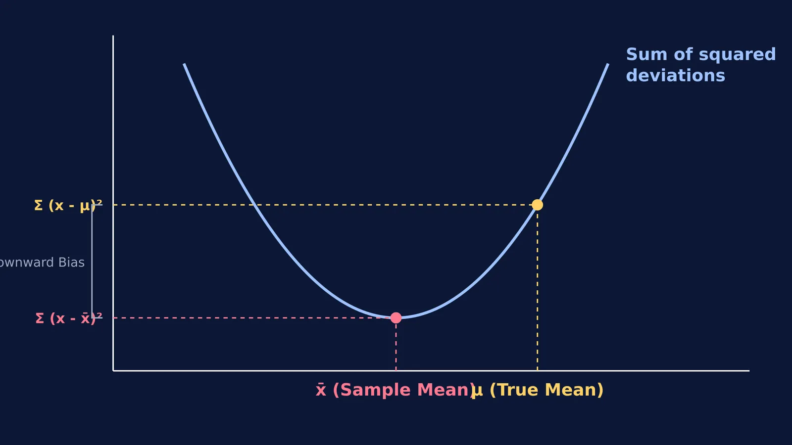
Using x̄ instead of μ introduces a hidden geometric catch: the sample mean is calculated directly from the observed data points. A foundational algebraic property of the arithmetic mean is that the sum of squared differences Σ(xᵢ − c)² reaches its absolute minimum value when c = x̄. If you replace x̄ with any other number—including the true population mean μ—the sum of squared deviations grows larger:
Σ(xᵢ − μ)² = Σ(xᵢ − x̄)² + n(x̄ − μ)²
Because the term n(x̄ − μ)² is always positive whenever x̄ differs from μ, the squared deviations measured around the sample mean are strictly smaller than the squared deviations around the true population mean. As Carl Friedrich Gauss proved in Article 38 of his 1823 treatise *Theoria combinationis observationum erroribus minimis obnoxiae*, taking the mathematical expectation across all possible samples yields E[Σ(xᵢ − x̄)²] = (n − 1)σ². If you divide this sample sum by n, your average result will equal ((n − 1)/n)σ². For a sample of 5 items, dividing by n underestimates the true population variance by 20%. As mathematician Felix Reichel notes in a 2025 study in the *Journal of Mathematics and Statistics*, applying Bessel's correction of n − 1 removes this downward bias in sample variance caused by using the sample mean.
Why does sample variance divide by n − 1 instead?
To eliminate this systematic underestimation, statisticians apply Bessel's correction, named after German astronomer Friedrich Wilhelm Bessel. Multiplying the biased sample variance by n/(n − 1) cancels out the bias factor, changing the divisor from n to n − 1:
s² = (1/(n − 1)) Σ(xᵢ − x̄)²
Taking the expected value confirms that E[s²] = σ², making s² an unbiased estimator of population variance.
Statisticians also describe this adjustment through degrees of freedom. A sample of n independent measurements contains n independent pieces of information. However, calculating the sample mean imposes a strict linear constraint: the sum of deviations around x̄ must always equal zero, Σ(xᵢ − x̄) = 0. Once you know any n − 1 deviations, the last one is fixed automatically. You only have n − 1 independent pieces of information left to estimate variability. Dividing by n − 1 scales the sum by the true degrees of freedom available.
When calculating sample variance computationally, standard formulas can introduce subtle rounding errors. In *The American Statistician*, Tony F. Chan, Gene H. Golub, and Randall J. LeVeque showed that multi-step summation algorithms are essential to avoid catastrophic numerical cancellation when evaluating (xᵢ − x̄)². Similar care is needed when correcting mean and variance after a wrong observation is fixed.
What formula do CBSE and board exams expect?
For school examinations, the decision is straightforward: always use the formula dividing by n.
Board marking schemes evaluate whether you understand descriptive statistics for finite data sets. Unless an exam question explicitly specifies an "unbiased sample variance" or mentions inferential sampling, you must divide by n for ungrouped data and by N = Σfᵢ for grouped frequency distributions. Competitive exams such as JEE Main adhere strictly to the same NCERT convention, including when calculating the variance of two combined groups.
When practising multi-step statistics questions, the Fermi Problem Library provides worked problems with a step-by-step solver that explains the reasoning rather than printing an answer. To explore how dispersion connects to probability distributions and higher-level data modelling, the Fermi Concept Library covers every concept in physics, chemistry, biology, mathematics and computing, each with its own lesson and its place in the map.
How does dividing by n compare to n − 1 in practice?
Consider a simple data set of 5 measurements: 2, 4, 4, 5, and 10.
Find the sample mean: x̄ = (2 + 4 + 4 + 5 + 10) / 5 = 25 / 5 = 5.
Calculate deviations from the mean: (2 − 5) = −3; (4 − 5) = −1; (4 − 5) = −1; (5 − 5) = 0; (10 − 5) = 5.
Square each deviation: 9, 1, 1, 0, and 25.
Sum the squared deviations: 9 + 1 + 1 + 0 + 25 = 36.
Now apply both formulas:
Population variance (CBSE / NCERT): σ² = 36 / 5 = 7.2.
Sample variance (Bessel's correction): s² = 36 / (5 − 1) = 36 / 4 = 9.0.
Notice the exact ratio: 7.2 / 9.0 = 4 / 5 = 0.8, which matches the predicted theoretical bias factor of (n − 1)/n = 4/5.
Use this rule of thumb whenever you calculate variance:
School exams (CBSE, ICSE, State Boards): divide by n.
Scientific calculators: select σn (or σx) for board exams; select sn (or sx) for experimental sample statistics.
Laboratory experiments: divide by n − 1 when estimating the random error of your apparatus across an infinite population of repeated trials.


