On this page
If every student in a class gets five bonus marks, the class average goes up by five. But does the spread of the marks change? What if you double everyone's score instead?
Understanding how shifting or scaling data affects the mean and variance is a standard part of high school statistics, and a common question in exams like the JEE Main.
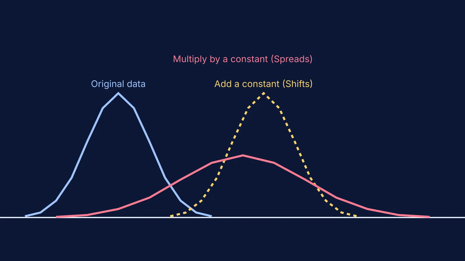
When adding a constant to data, the variance remains unchanged (e.g., adding 5 grace marks leaves variance at 25). However, multiplying by a constant scales the variance by that number squared, so doubling the scores quadruples the variance to 100.
What is the effect of adding a constant on mean and variance?
Adding a constant to every observation is mathematically called a change of origin. Imagine a set of exam scores where the mean is 40 and the variance is 25 (meaning the standard deviation is 5).
If the teacher awards 5 grace marks to every student, every single data point slides 5 units to the right on the number line.
The mean: The new mean is simply the old mean plus the constant. The expected value operator is linear, so adding a constant increases the mean by that constant. The average becomes 40 + 5 = 45.
The variance: The variance measures how far the scores are spread out from the mean. Adding a constant to all values of a variable leaves the variance unchanged. Because every score shifted by the exact same amount, the distances between the scores have not changed, and the variance remains 25.
Why does the variance stay the same when adding?
To understand why the spread remains identical, you have to look at the mathematical definition of variance. Variance is calculated as the average of the squared differences from the mean.
Let's trace what happens to a single data point, x, when we add a constant a. The new data point becomes x + a. As we established, the new mean becomes x̄ + a.
When you calculate the distance between the new data point and the new mean, the constant a cancels out entirely: (x + a) − (x̄ + a) = x − x̄.
Since the difference from the mean for every single point is exactly the same as it was before the shift, the squared differences are the same, and their average is the same. The mathematical spread is identical, even though the actual values are higher.
How does multiplying by a constant change the variance?
Multiplying every observation by a constant is called a change of scale. Suppose the teacher decides to double every score instead of adding 5.
The mean: The new mean is multiplied by the constant. The average becomes 40 × 2 = 80.
The variance: Multiplying stretches the data out. A student who was 5 marks above the old mean is now 10 marks above the new mean. Multiplying all values by a constant scales the variance by the square of that constant. The new variance becomes 25 × 2² = 100.
The standard deviation, which is the square root of the variance, simply gets multiplied by the absolute value of the constant. In this case, the standard deviation goes from 5 to 10.
Why does the variance square the multiplier?
If we multiply our original data point x by a constant h, the new point is hx. The new mean also scales, becoming hx̄.
The new distance from the mean for this point is hx − hx̄. If you factor out the constant, this distance is h(x − x̄).
Because variance requires us to square these distances, we must square the entire expression. Squaring h(x − x̄) gives us h²(x − x̄)². Every single squared distance is multiplied by h². Consequently, when you take the average of all these new squared distances to find the variance, the final result is exactly h² times the original variance.
What happens when you combine adding and multiplying?
In many real-world scenarios, such as converting temperatures from Celsius to Fahrenheit or scaling exam scores to a new grading system, you must apply both operations simultaneously. This is known as a linear transformation, often written in the form y = ax + b, where a is the multiplier and b is the constant you add.
When you apply a linear transformation to a dataset, you simply combine the two rules we have just covered. The new mean will be affected by both the multiplication and the addition. If your original mean is x̄, your new mean becomes ax̄ + b.
However, because adding a constant has absolutely no effect on the spread of the data, the new variance is completely unaffected by the constant b. It is only affected by the multiplier a. Therefore, the new variance becomes a² times the original variance. The standard deviation, similarly, is multiplied by the absolute value of a, and ignores b entirely.
This combined rule is incredibly useful because it means you do not have to recalculate the variance from scratch for the new dataset. You only need to know the original variance and the scale factor.
Seeing the change with sliders
It is one thing to memorise the rules and algebra, but seeing the distribution change makes it intuitive. If you want to see this in motion, the Fermi Simulation Lab has interactive simulations for the ideas that are easier to see than to read. You can drag a slider to add a constant to a set of points and watch the entire curve slide to the right without changing shape. Then, you can drag the multiplication slider to see the curve spread out and flatten as the variance increases.
For more practice with how the formula works, you can read How adding to or scaling data changes the mean and variance. If you are looking at two separate classes rather than changing one class's scores, you will need the variance of two combined groups instead.