On this page
Two cells, one wire, two lengths where the galvanometer reads zero: that is the whole comparison. A simulation helps most with the next step: predicting where the null points move when you change the wire or the driver cell.
How does a potentiometer compare two EMFs?
A driver cell sends a steady current through a long, uniform wire, so the potential falls evenly along it. OpenStax College Physics 2e describes the potentiometer as a voltage source that "passes a constant current through" a long wire, with a sliding contact moved until the galvanometer reads zero.
At that null point no current flows through the cell being tested, so the voltage across it equals its EMF. OpenStax writes the result as emf_x/emf_s = R_x/R_s, and because the wire is uniform, that ratio of resistances equals the ratio of the balancing lengths.
In symbols: E1/E2 = l1/l2. The potential gradient k (volts per centimetre) cancels out, so you never need the driver cell's EMF. OpenStax notes that the uncertainty "can be considerably smaller than when using a voltmeter directly, but it is not zero." If EMF still feels slippery, read why EMF is not a force first.
How do you find the balancing length in a simulation?
Connect the driver cell, a rheostat and the wire in series, with the driver's positive terminal at the zero end (A) of the wire.
Connect cell 1's positive terminal to A as well, and its negative terminal through the galvanometer to the jockey.
Touch the jockey near A, then near the far end B. The needle should swing opposite ways. If it swings the same way both times, a terminal is reversed or the driver is too weak.
Close in on the point of zero deflection and record l1.
Switch the two-way key to cell 2 and record l2.
Worked example: what numbers should you expect?
These are simulation settings chosen for easy arithmetic: a 2.0 V driver with negligible internal resistance, a 2 ohm rheostat, a 400 cm wire of resistance 8 ohm, E1 = 1.5 V and E2 = 1.0 V.
Current: 2.0 / (8 + 2) = 0.2 A.
Drop across the wire: 0.2 x 8 = 1.6 V, so k = 1.6 / 400 = 0.004 V/cm.
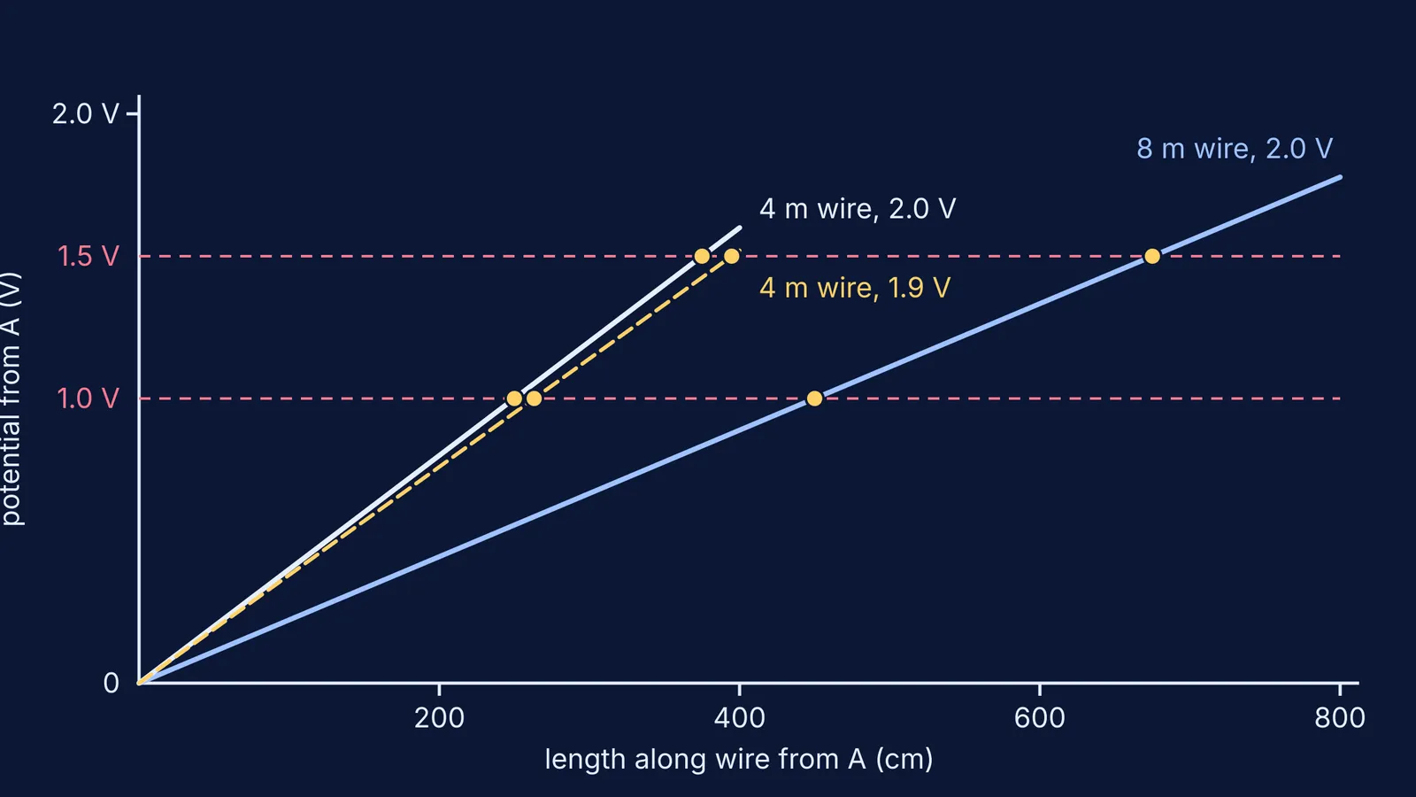
l1 = 1.5 / 0.004 = 375 cm and l2 = 1.0 / 0.004 = 250 cm.
l1/l2 = 1.5, the same as E1/E2.
What happens to the null point with a longer wire or a weaker driver cell?
Write down a prediction before each change.
Longer wire. Double the wire to 800 cm of the same material, so its resistance doubles to 16 ohm (our post on how length and thickness set a wire's resistance explains why). The current becomes 2.0 / 18, about 0.111 A, the drop is about 1.78 V and k is about 0.00222 V/cm. The null points move out to 675 cm and 450 cm; the ratio is still 1.5. A 1 mm reading error is now a smaller fraction of each length, so the comparison is more precise.
Weaker driver cell. Keep the 400 cm wire and drop the driver to 1.9 V. The current is 0.19 A, the drop is 1.52 V and k = 0.0038 V/cm. The null points move to about 394.7 cm and 263.2 cm. Both shift away from A; the ratio is again 1.5.
Too weak. Now set the driver to 1.8 V. The drop across the whole wire is 1.44 V, less than E1 = 1.5 V, so cell 1 has no null point anywhere on the wire and the needle deflects the same way at both ends. Cell 2 still balances, at about 277.8 cm. The rule: the drop across the full wire must be larger than every EMF you want to compare.
If you would rather watch the gradient change than calculate it, the Fermi Simulation Lab has interactive simulations for ideas that are easier to see than to read. When a result surprises you, Fermi's AI tutor can run the simulation with you and check your understanding as it goes.
Is the potentiometer still in the CBSE Class 12 syllabus?
The CBSE Class 12 physics syllabus for 2025-26 lists Current Electricity topics up to Kirchhoff's rules and the Wheatstone bridge, with no potentiometer in the theory, and its Section A experiments use a metre bridge rather than a potentiometer. It does keep an activity "to study the variation in potential drop with length of a wire for a steady current", the idea the whole method rests on.
If your board or entrance exam covers the potentiometer, check its current official syllabus. Either way, the three predictions above test whether you understand potential gradient. For a routine, see our guide to predicting first, then testing with AI and a simulation.