On this page
You can find π with a square, a quarter circle and a lot of random numbers. Here is how it works, how to predict your result, and why the last digits are so expensive.
How do random points estimate pi?
Take a square with side 1 and draw a quarter circle of radius 1 centred on one corner. The square has area 1 and the quarter circle has area π/4, so a point placed uniformly at random in the square lands inside the quarter circle with probability π/4. Count the fraction of points that land inside and multiply by 4: that is your estimate of π, the example used in the Wikipedia article on the Monte Carlo method.
Testing a point needs no square root: a point (x, y) is inside the quarter circle when x² + y² ≤ 1.
This is a Monte Carlo method, which answers a numerical question by repeated random sampling. Nicholas Metropolis and Stanisław Ulam described the approach in a 1949 paper titled The Monte Carlo Method in the Journal of the American Statistical Association. You can read how a card game led Ulam to the idea in how a game of solitaire invented the Monte Carlo method, and meet an older cousin of this experiment in Buffon's needle problem.
A worked example with 40 points
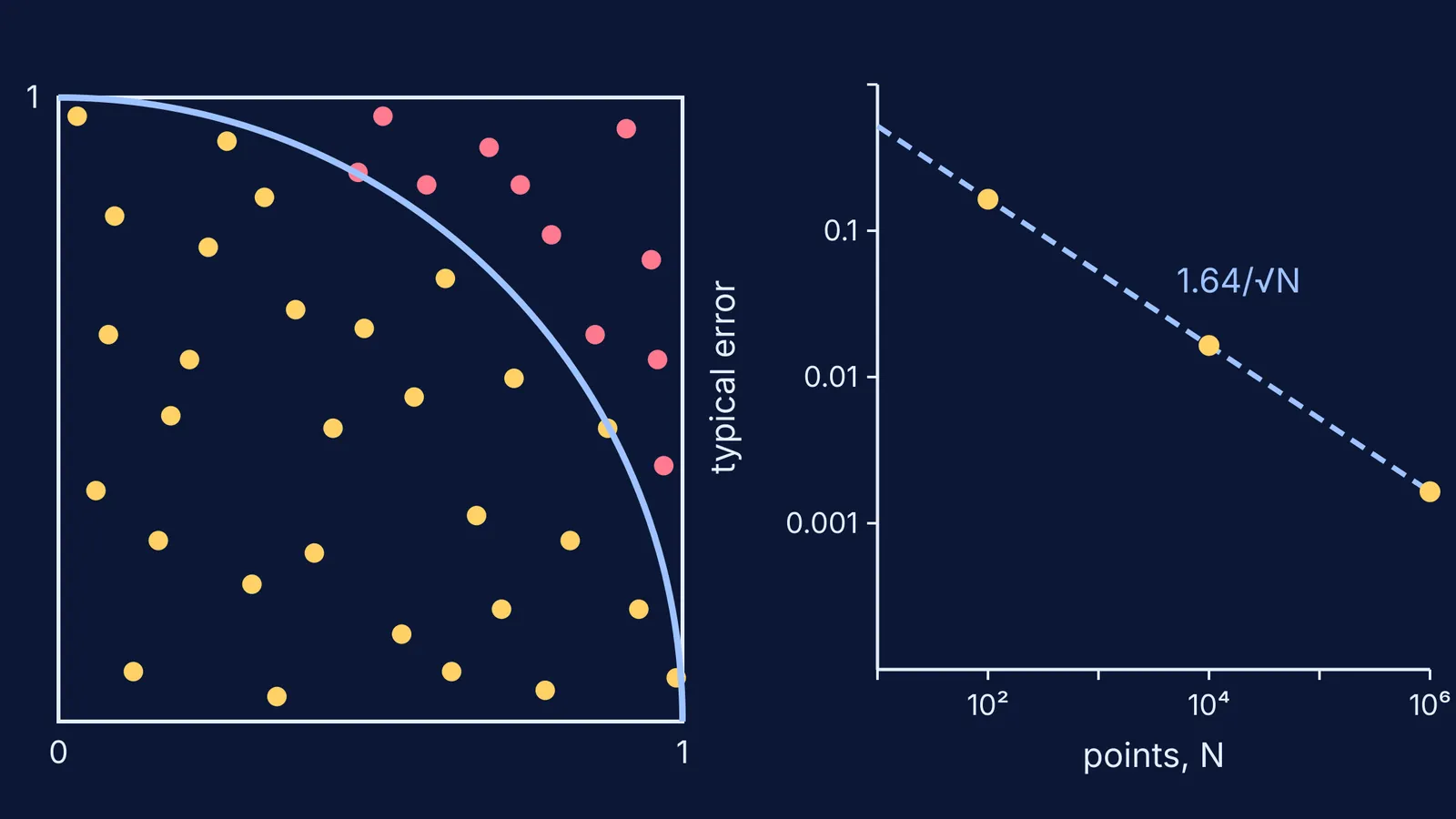
The diagram at the top applies the quarter-circle test to 40 hand-placed points: for each, square both coordinates and add them. Two sit right on the edge:
(0.88, 0.47) gives 0.7744 + 0.2209 = 0.9953, so it is just inside.
(0.48, 0.88) gives 0.2304 + 0.7744 = 1.0048, so it is just outside.
Of the 40 points, 29 land inside. The estimate is 4 × 29/40 = 2.9, about 0.24 below π. Did something go wrong? You can answer that before counting a single point.
How accurate is the estimate with N points?
Each point is a yes-or-no trial that hits with probability p = π/4 ≈ 0.785. Score a hit as 4 and a miss as 0, and the standard deviation of one point's score is 4√(p(1 − p)) ≈ 1.64. Stefan Weinzierl's lecture notes show that the error of a Monte Carlo estimate is on average σ/√N, where σ is that standard deviation and N is the number of samples (Weinzierl, Introduction to Monte Carlo methods). So the typical error of your π estimate is about 1.64/√N:
40 points: about ±0.26
100 points: about ±0.16
1,000 points: about ±0.052
10,000 points: about ±0.016
1,000,000 points: about ±0.0016
The same notes use the central limit theorem to show that, for large N, repeated estimates spread out in a bell curve. For a bell curve, about 68% of values lie within one standard deviation of the mean and 95% within two (the 68–95–99.7 rule). The 40-point result of 2.9 is 0.24 below π, inside one typical error. Nothing went wrong; that is normal luck for 40 points.
Why does the Monte Carlo error shrink so slowly?
Because of the square root. As the Monte Carlo method article puts it, quadrupling the number of sampled points halves the error. One more correct decimal place needs an error ten times smaller, which takes 100 times as many points. To pin π to about ±0.01 you need roughly (1.64/0.01)² ≈ 27,000 points; for ±0.001, about 2.7 million.
Compare that with how Archimedes trapped π between 223/71 and 22/7, which tightens by geometry rather than luck. Weinzierl's notes call Monte Carlo convergence relatively slow but name its strength: the 1/√N error does not depend on the number of dimensions of the integral.
Try it: a predict-then-run plan
You can run this in Google Sheets, where RAND() returns a random number from 0 up to but not including 1 (Google Sheets RAND help).
In A1 type =RAND(), in B1 type =RAND(), and in C1 type =IF(A1^2+B1^2<=1,1,0).
Copy row 1 down to row 100. In E1 type =4*AVERAGE(C1:C100).
Before you look, write your prediction: with 100 points, about 2 runs in 3 should land between 2.98 and 3.31.
Make 10 fresh runs and write down E1 each time. RAND is a volatile function, and in automatic mode Sheets applies changes as soon as you make a spreadsheet action, so any edit gives a fresh run (Google Sheets calculation settings). Count how many runs fall in your range.
Copy the rows down to row 10,000 and change E1 to =4*AVERAGE(C1:C10000). Predict first: the spread should shrink by 10 times, to roughly 3.125 to 3.158, not by 100 times.
Work out how many rows you would need to trust the third decimal place.
Ten runs is a small sample too, so 5 or 9 in range still fits the prediction. If you get 2, check column C.
The Fermi Simulation Lab has interactive simulations for ideas that are easier to see than to read. If standard deviation is the shaky step, the Fermi Concept Library gives each concept in mathematics its own lesson and its place in the map.