On this page
You cannot count every fish in a lake. Mark and recapture gets around this with two samples and one ratio. The method is old: C.G.J. Petersen used it on plaice in 1896, and F.C. Lincoln used it on waterfowl in 1930, which is why the basic formula carries both their names (overview of mark and recapture).
India's national tiger survey uses a camera-trap version of it. In the 2022 survey, camera traps were placed at 32,588 locations for mark recapture analysis, and 3,080 unique tigers were photographed, giving a minimum estimated population of 3,167 (NTCA and Wildlife Institute of India summary report). There a camera photo does the job of the tag.
How does the mark and recapture method work?
Catch a first sample, mark every animal, and count them. Call this M.
Release them and let them mix back into the population.
Catch a second sample. Count everything you caught (C) and how many of those carry a mark (R).
Estimate the total: N = M × C ÷ R. This is the Lincoln-Petersen formula (formula and assumptions).
The logic is a proportion: if tagged fish mix in evenly, the tagged share of your second catch (R ÷ C) matches the tagged share of the lake (M ÷ N).
How do you calculate population size with the Lincoln-Petersen formula?
Use a virtual pond, so you know the true answer. Put 500 fish in it, tag 50, release them, then catch 50. One fish in ten is tagged, so you expect about 5 tagged fish in your catch. If you get exactly 5: N = 50 × 50 ÷ 5 = 500. Correct.
Statisticians also use the Chapman version, N = (M + 1)(C + 1) ÷ (R + 1) − 1, which is less biased when samples are small (Chapman estimator). With R = 5 it gives about 432. That is not a mistake: Chapman is built to be less biased on average over many repeats, not to hit the answer in any single catch.
Why do small samples give wrong estimates?
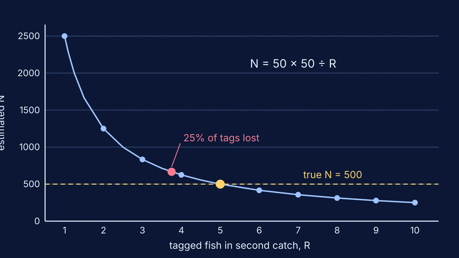
The Lincoln-Petersen estimate is biased at small sample sizes and only becomes unbiased as samples grow very large (bias of the estimator). In the 50-and-50 pond, every estimate is 2,500 ÷ R, so one fish more or less swings the answer a lot:
R = 6 gives 417
R = 5 gives 500
R = 4 gives 625
R = 3 gives 833
R = 2 gives 1,250
R = 0 means dividing by zero: no estimate at all
Shrink the samples to 10 and 10 and you expect only 0.2 tagged fish per catch; by our own calculation, roughly four catches in five contain none. Polls face the same problem; see how sample size sets the margin of error.
What happens to the estimate when tags fall off?
A fish that lost its tag looks unmarked. So R comes out too small and N comes out too big. A 2011 study in Transactions of the American Fisheries Society states that, unless accounted for, tag loss will cause mark-recapture methods to overestimate the true abundance of a closed population and underestimate the uncertainty (Hyun, Reynolds and Galbreath, 2011). In their study of kokanee salmon in Oregon's Metolius River in 2007, they estimated a tag loss rate of 0.27.
In the virtual pond, if a quarter of the 50 tags fall off, you expect 3.75 tagged fish per catch and an estimate of 2,500 ÷ 3.75, about 667. That is a third too high. In general, the estimate drifts to roughly true N ÷ (1 − fraction of tags lost).
Keeping tags on is one of the method's core assumptions. The others: the population is closed (no births, deaths or migration between samples), marks are recorded correctly, and every animal is equally likely to be caught (assumptions of the method).
How can you test mark and recapture with a simulation?
A jar of 500 dried chickpeas and a marker pen works as the pond; so does a spreadsheet with a random number function.
Baseline: true N = 500, tag 50, catch 50. Repeat 20 times and write down each estimate.
Small samples: tag 10, catch 10. Count how often R = 0 and how wild the other estimates are.
Large samples: tag 150, catch 150. Your 20 estimates should bunch much closer to 500.
Lost tags: with 150 and 150, wipe the mark off a quarter of the tagged chickpeas before the second catch. Watch the estimates bunch around 667 instead.
Compare: work out both Lincoln-Petersen and Chapman for every run and average them.
If you would rather watch the pattern than count chickpeas, the Fermi Simulation Lab is where we put interactive simulations for ideas that are easier to see than to read. If the formula still feels like a trick, Fermi's AI tutor works out what you already know and builds a plan for the session.
Next, see population growth rate calculations and genetic drift in a small population, simulated.