On this page
Picture two ponds, one with ten frogs and one with a thousand, and two frog colours that are equally fit. In the small pond one colour is often gone within a few dozen generations; in the big pond both survive far longer. Nothing selected against the colour that vanished. Chance did it, and chance here comes with formulas, so you can predict a drift simulation before you run it.
What is genetic drift in a simulation?
Genetic drift is the tendency for allele frequencies to change from one generation to the next in a finite population even if there is no selection, as Kent Holsinger defines it in his University of Connecticut population genetics notes.
A standard drift simulation, often called the Wright-Fisher model, follows the recipe in those notes. A population of N diploid individuals carries 2N copies of a gene, and each new generation is built by drawing 2N copies at random from the parents' gene pool. Think of tossing a coin 2N times, where the chance of heads is the allele's current frequency.
Because each generation is a random sample, the frequency wobbles, with a variance of p(1 − p)/2N. The smaller the population, the bigger each random step.
How fast is an allele lost or fixed in a small population?
Three results from Holsinger's notes let you make predictions:
Which allele wins: the probability that an allele is eventually fixed equals its current frequency. Start at 50% and it is a coin flip; start at 10% and it is lost nine times in ten.
How long it takes: the average time until one allele or the other is fixed is about −4N[p ln p + (1 − p) ln(1 − p)] generations. At p = 0.5 this is 4N ln 2, roughly 2.8N.
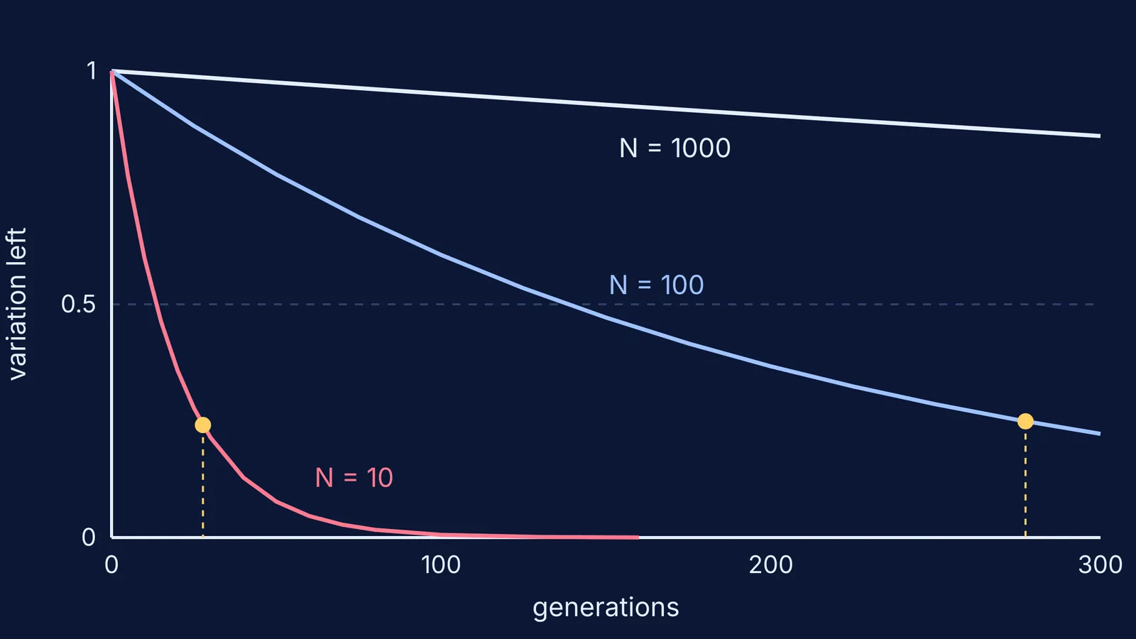
How fast variation fades: the expected share of heterozygosity left after t generations is (1 − 1/2N)^t, so a population of 10 loses 5% of its remaining variation every generation.
The same fixation rule covers a brand-new mutation present as a single copy: its chance of ever taking over is 1/2N, its starting frequency.
Worked example: predict before you press run
Set one allele at 50%, no selection. Before running, write down these predictions from the formulas in Holsinger's notes:
N = 10 (20 gene copies). Average time to fixation or loss: 4 × 10 × ln 2 ≈ 28 generations. Variation left after 20 generations: 0.95^20 ≈ 36%. A single new mutant has a 1 in 20 (5%) chance of ever taking over.
N = 100 (200 copies). Average time: about 277 generations. Variation left after 20 generations: 0.995^20 ≈ 90%. A single new mutant's chance: 0.5%.
N = 1,000 (2,000 copies). Average time: about 2,800 generations. Variation left after 20 generations: about 99%. A single new mutant's chance: 0.05%.
Now start at 10% with N = 10. The formula gives about 1.3N, roughly 13 generations, with the allele lost in about 90% of runs. Rare alleles are settled faster, mostly by vanishing.
Then run it. One run can miss these averages by a lot, so run many populations side by side, count fixations and losses, and compare.
Did real populations behave like the simulation?
Peter Buri tested this with fruit flies and published the results in Evolution in 1956. He set up two series of 107 and 105 bottles, each started with two eye-colour alleles, bw75 and bw, at a frequency of 0.50. Every generation, for 19 generations, he picked 16 flies from each bottle, 8 males and 8 females, to found the next one.
Buri found no evidence of selection in either series, but the bottles drifted faster than 16 flies would predict: his estimates of effective population size were 9.0 and 11.5, which is 56% and 72% of the 16 flies used. He associated the lower figure with severe crowding in the smaller vials of the first series.
The lesson for any simulation: N in the formulas is the effective size, often smaller than a head count. For the history, read our post on Sewall Wright and genetic drift.
How should you use a drift simulation to study evolution?
Drift often sits next to natural selection and Hardy-Weinberg equilibrium in school evolution chapters (see our guide to evolution for NEET). A short routine:
Write your prediction first, using the worked example above.
Change one thing at a time: N or the starting frequency.
Explain each result in one sentence that uses the word "sampling".
Link it to Hardy-Weinberg: drift is what happens when the large-population assumption fails.
For when moving pictures help and when they don't, see our look at simulations or static diagrams.
For other ideas that are easier to see than to read, the Fermi Simulation Lab has interactive simulations, and the Fermi Concept Library gives each biology concept its own lesson and its place in the map.
Pick a population of 10, set the allele to 50%, write down "about 28 generations", and press run.