On this page
Make one dot swing left-right and up-down at once. The path it leaves is a Lissajous figure, and three numbers let you predict it before you press play.
What are Lissajous figures?
Lissajous figures are curves produced when the x and y coordinates of a point are each given by a sine wave, which may have any amplitude, frequency and phase, as the UNSW School of Physics page on Lissajous figures puts it.
Nathaniel Bowditch studied these curves in 1815, and Jules-Antoine Lissajous studied them in more detail, independently, in 1857, according to Wolfram MathWorld. The same MathWorld entry states that the curve is periodic only if the ratio of the two frequencies is rational; otherwise it never repeats.
Here are the equations we will use:
x = A sin(ω₁t)
y = B sin(ω₂t + φ)
Each line alone is simple harmonic motion; if that is shaky, start with our simple harmonic motion simulation and its five predictions. The ratio ω₁:ω₂ sets how many lobes the figure has. The phase difference φ sets where y is in its cycle when x starts, which tilts, fattens or folds the shape.
How do you make Lissajous figures?
A simulation or graphing tool. Enter x and y as parametric equations, run t from 0 to 2π, and put φ on a slider.
An oscilloscope in X-Y mode. Feed one sine signal to the x input and another to the y input. Durham University's physics lab guide notes that the figure tells you the phase difference between the two signals and the ratio of their frequencies.
A harmonograph. Before electronics, pendulums swinging at different frequency ratios drew these curves mechanically, as the Wikipedia overview of Lissajous curves describes.
The Fermi Simulation Lab has interactive simulations for the ideas that are easier to see than to read, including oscillators.
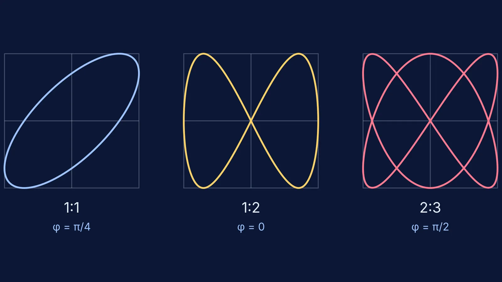
What pattern do you get for 1:1, 1:2 and 2:3?
Cover the answers below, sketch your guess for each case in about 20 seconds, then run it. We take A = B so the figure fits a square.
For a 1:1 ratio (same frequency):
φ = 0: a straight line through the centre, sloping up.
φ = π/4: an ellipse tilted along that same diagonal.
φ = π/2: an ellipse with its axes along x and y; with A = B it is a circle.
φ = 3π/4: an ellipse tilted along the other diagonal.
φ = π: a straight line sloping down.
For a 1:2 ratio (y oscillates twice as fast):
φ = 0: a figure of eight with one lobe on each side, crossing at the centre.
φ = π/4: still an eight, but the crossing point slides up the y-axis to about 0.71B and each lobe is no longer symmetric top to bottom.
φ = π/2: the eight folds into an arch. Using cos 2t = 1 − 2sin²t, you get y = B(1 − 2x²/A²), a parabola traced forwards and back.
For a 2:3 ratio:
φ = 0: a closed, knotted curve through the centre.
φ = π/4: the curve stops closing. It runs between two corners, (−A, B) and (−A, −B), and retraces itself.
φ = π/2: closed again, and mirror-symmetric about the vertical axis. This is the right-hand curve in the diagram at the top of this post.
Why does the phase difference change the shape?
At φ = 0 in the 1:1 case, x and y reach their peaks together, so the dot moves along a diagonal. Shift y by a quarter cycle (π/2) and y peaks when x is at zero, which opens the line into an ellipse.
At some phases both motions turn round at the same instant, so the dot runs out to an end and comes back along its own path. That is why 1:1 collapses to a line at φ = 0 and π, 1:2 becomes a parabola at π/2, and 2:3 opens at π/4.
A 15-minute prediction plan
Write both equations on paper and set A = B.
Sketch all eleven cases above before running anything.
Run each case and mark it right or wrong.
For each miss, do the wall-counting check and ask whether the phase made the curve open or closed.
Finally, predict 3:4 at φ = 0 without help, then test it.
If your curve looks jagged, the tool may be joining too few sampled points; our post on the limits of physics simulations explains why that happens and how to check. And if you let the amplitudes shrink over time, the figure spirals inward, which links to damped and forced oscillations.
Make your sketches first, then let your graphing tool tell you which ones you got right. For more ideas that are easier to see than to read, browse the Fermi Simulation Lab.