On this page
When a population expands, it follows predictable mathematical patterns. Biologists use these patterns to predict how a species will fare over time. The NCERT Class 12 Biology textbook highlights two primary models of population growth: exponential and logistic.
Whether you are preparing for exams or simply curious about ecology, comparing these models helps explain why some species take over an environment rapidly while others remain stable. You can use an AI tutor to break down the mathematics, plot the curves, and check your understanding against the textbook.
What is exponential population growth?
Exponential growth occurs when a species has access to unlimited resources, such as food and space. Under these ideal conditions, the population can realise its full innate potential to multiply.
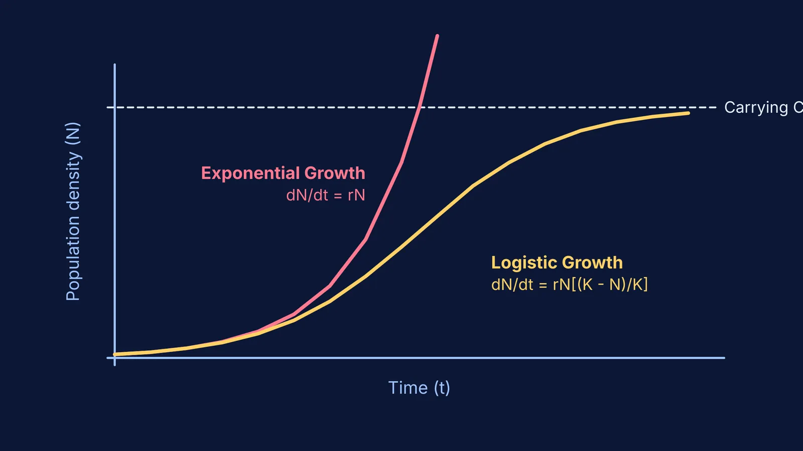
This model is described by the equation dN/dt = rN, where N is the population size, t is time, and r is the intrinsic rate of natural increase. Because the growth rate accelerates as the population gets larger, plotting this data yields a steep, J-shaped curve.
According to the NCERT Biology textbook, the intrinsic rate of natural increase (r) is 0.015 for the Norway rat and 0.12 for the flour beetle (Source). For context, the r value for the human population in India in 1981 was 0.0205.
Natural examples of exponential growth are often short-lived because resources eventually run out. Algal blooms in nutrient-rich ponds and insect populations exploding during the monsoon are classic examples. You can ask Fermi's AI tutor to run the simulation for these scenarios, letting you see exactly when a J-shaped curve becomes unsustainable.
What is logistic population growth?
In the real world, resources are rarely unlimited. As a population grows, competition for finite resources intensifies, and only the fittest survive. This reality is captured by the logistic growth model, which the NCERT textbook describes as the more realistic scenario for most wild animal populations.
The logistic model modifies the growth equation to include a carrying capacity (K), which is the maximum number of individuals the habitat can support. The equation becomes dN/dt = rN[(K - N)/K].
When you plot logistic growth, it forms a sigmoid or S-shaped curve. It starts with a lag phase, accelerates exponentially for a time, and then decelerates before flattening out as the population reaches K. A classic example is a yeast culture growing in a closed laboratory vessel: the yeast multiply rapidly at first, but growth stalls as nutrients are depleted and waste builds up.
How do population interactions affect growth?
No population exists in isolation. Species interact constantly through predation, competition, parasitism, and mutualism. These interactions determine both the intrinsic growth rate and the environment's carrying capacity.
For instance, if a forest supports a population of herbivores, their carrying capacity is limited not just by the grass they eat, but also by the predators that hunt them. If you are solving ecology problems that involve changing these variables, the Fermi Problem Library can walk you through the reasoning step by step.
Checklist for exam prep
When checking your understanding against the syllabus, ensure you can:
Write both differential equations from memory.
Identify which curve is J-shaped (exponential) and which is S-shaped (logistic).
Explain why the logistic model is more realistic in nature.
Define carrying capacity (K) and intrinsic rate of natural increase (r).
When studying these topics, it is useful to connect the biological concepts to the underlying mathematics. To see how these differential equations govern other systems, read our guide on population growth and cooling. For an example of how ecological systems handle accumulation, see our explanation of biological magnification.