On this page
In 1988, Vasant Gowariker, then secretary of the Department of Science and Technology, worked with meteorologists from the India Meteorological Department (IMD) and the Indian Institute of Tropical Meteorology, Pune, on a model built from 16 temperature, pressure, wind and snow-cover signals from across the world (Down To Earth, 1992). Gowariker (1933 to 2015) was a rocket propellant scientist who directed the Vikram Sarabhai Space Centre from 1979 to 1985 (Wikipedia).
India's long-period average monsoon rainfall is 89 cm, with a year-to-year variation of about 10%, and even that swing can hurt farms (Rajeevan et al., Climate Dynamics). For why the monsoon arrives at all, see what drives the Indian monsoon winds.
What was the Gowariker power regression model?
It was two models in one paper. In 1989, in IMD's journal Mausam, Gowariker and four co-authors described a parametric model that gave a qualitative forecast and a power regression model that gave a number (Gowariker et al., 1989). That first version used 15 signals in four groups:
Temperature: El Niño, plus land temperatures in India and the northern hemisphere
Wind: the April 500 hPa ridge over India and two high-altitude wind patterns
Pressure: Darwin, Tahiti minus Darwin, Argentina and the equatorial Indian Ocean
Snow cover: the Himalayas and Eurasia
A 1991 follow-up described the 16-parameter power regression model that IMD used operationally, and argued that a forecast from one to four parameters cannot be reliable on all occasions (Gowariker et al., 1991).
The power regression equation has the form R = c₀ + Σ cᵢ Xᵢ^pᵢ, where R is monsoon rainfall, each X is a signal, and the c and p values are constants fitted to past data (Gowariker et al., 1989). The team fitted the constants on 23 years of data (1958 to 1980), and the powers ranged from +4 to −4. In plain words: each signal gets its own weight and curve, because rainfall does not rise in a straight line with, say, snow cover.
How did counting the signals work?
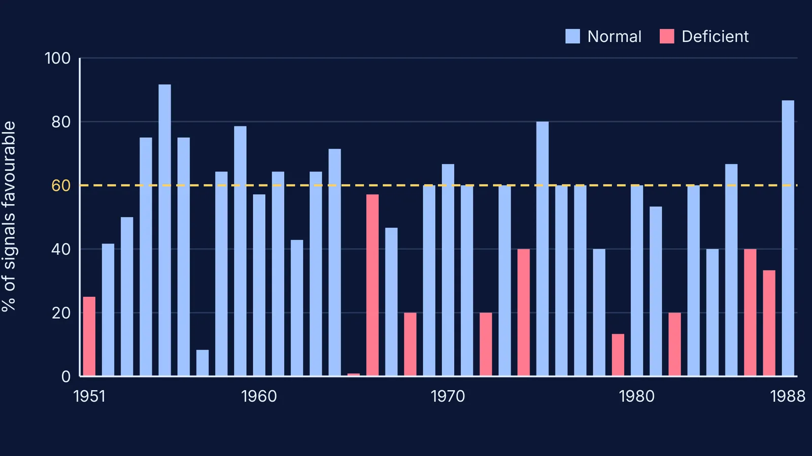
The parametric model works by hand: mark each signal favourable or unfavourable for a normal monsoon, then count. From 1951 to 1987 there were 18 years in which 60% or more of the signals were favourable, and the monsoon was normal in all 18 (Gowariker et al., 1989). In 1965 not one signal was favourable, and rainfall came in at 79% of normal. A high count was a "sufficient condition", not a necessary one: in 1957 only 1 of 12 signals was favourable, yet the monsoon was normal.
Worked example: forecast a monsoon like it is 1988
Repeat the parametric step with numbers from the paper's Table 1 (Gowariker et al., 1989).
Count the favourable signals. 1988: 13 of 15. 1974: 6 of 15. 1966: 8 of 14.
Turn each count into a percentage. 13 ÷ 15 = 87%. 6 ÷ 15 = 40%. 8 ÷ 14 = 57%.
Compare with the 60% line. Only 1988 clears it, so only 1988 gets a confident "normal" call.
Check what happened. 1988 was normal; 1974 and 1966 were both deficient.
Notice the grey zone. Below 60%, the table has both outcomes: 1960 had 57% favourable and was normal, while 1966 had the same 57% and was deficient.
Step 5 is why the team also built the quantitative model. It uses the least-squares fitting you meet in linear regression with Class 11 maths, with a curved term for each signal instead of a straight line.
How accurate was the 16-parameter model, and why was it dropped?
It started well. In test years kept out of the fitting (1981 to 1988), the power regression forecast had a root mean square error of 5.6 cm, nearly 6% of normal rainfall, and it correctly called the droughts of 1982, 1986 and 1987 (Gowariker et al., 1989). Operationally, it forecast 102% of normal for 1989 (actual: 101%) (Down To Earth).
The longer record was mixed. IMD scientists later wrote that the 16-parameter forecasts from 1988 to 2002 were qualitatively correct, but their average error was larger than that of forecasts based on the long-term average alone, and the model failed to predict the severe drought of 2002 (Rajeevan et al., Climate Dynamics). In 2003, IMD moved to new 8- and 10-parameter models and a two-stage forecast, issued in April and updated by the end of June. After a failed 2004 forecast, IMD scientists revisited the predictors again, partly because the monsoon's link with El Niño had weakened. Seasonal totals also hide what happens within a season, as Sulochana Gadgil's work on the northward-pulsing rain band shows.
What can you learn from Gowariker's model?
Many weak signals, each weighted, can carry more information than one strong-looking cause.
Test on years the model has never seen.
A good past fit is not future skill. Relationships can drift.
If exponents or least squares are the shaky part, the Fermi Concept Library gives each mathematics concept its own lesson and shows its place in the map.
Next time IMD issues its April monsoon forecast, you will know where its statistical side began.