
On this page
Pulsars were announced in Nature on 24 February 1968. Within about a year, as R. N. Manchester recounts in Pulsars at Parkes, V. Radhakrishnan and colleagues had measured the polarisation of the Vela pulsar, and Radhakrishnan and D. J. Cooke explained it with what became the rotating vector model. Manchester writes that these observations strongly supported the picture of a rotating neutron star whose beam points outward from a magnetic pole.
Who was V. Radhakrishnan?
Venkatraman Radhakrishnan (1929–2011) was the son of C. V. Raman and directed the Raman Research Institute in Bengaluru from 1972 to 1994, according to his Wikipedia biography.
In 1968 and 1969 he was working with the Parkes 64-metre radio telescope in Australia (Manchester 2018). Manchester recalls being asked to help "Rad" with the Vela pulsar observations. For the story of how pulsars were found in the first place, read our piece on Jocelyn Bell Burnell and the discovery of pulsars.
What did Radhakrishnan and Cooke see in the Vela pulsar?
Radio waves, like light, can be linearly polarised: the electric field oscillates along one direction, and astronomers call the angle of that direction on the sky the position angle. Our Malus's law polariser simulation is a quick refresher on polarisation.
At Parkes, the Vela pulsar's pulses turned out to be very strongly linearly polarised, and the position angle did not stay put: it swung steadily through each pulse. In the 1969 data reproduced in Pulsars at Parkes, the angle runs from 205° at one edge of the pulse to 25° at the other, a turn of 180°. Manchester's later account adds that the swing looked the same at different radio frequencies.
What is the rotating vector model?
A pulsar's magnetic field is close to that of a bar magnet, so seen from above a magnetic pole its field lines fan out like the spokes of a wheel. In the model, radiation is emitted along the field lines and is linearly polarised in the plane in which each field line curves (Manchester 2018). Manchester cites the paper as Astrophysical Letters, volume 3, pages 225–229.
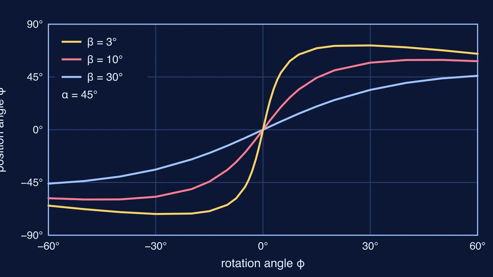
As the star spins, your line of sight sweeps across that fan of spokes, so the polarisation angle you measure turns with them. The model predicts that the swing is most rapid when the line of sight passes close to the magnetic axis (Pulsars at Parkes).
In symbols, as written by Everett and Weisberg (2001): tan(ψ − ψ₀) = sin α sin(φ − φ₀) / (sin ζ cos α − cos ζ sin α cos(φ − φ₀)). Here φ is how far the star has rotated, α is the angle between the spin axis and the magnetic axis, ζ is the angle between the spin axis and your line of sight, and β = ζ − α is how close your line of sight comes to the magnetic axis. The steepest slope of the curve is sin α / sin β.
How do you read an S-shaped polarisation curve?
A worked example with Everett and Weisberg's slope formula and α = 45° (the three curves in the diagram above):
β = 3°: steepest slope = sin 45° / sin 3° = 0.707 / 0.052 ≈ 13.5° of position angle per degree of rotation.
β = 10°: 0.707 / 0.174 ≈ 4.1° per degree.
β = 30°: 0.707 / 0.500 ≈ 1.4° per degree.
To read a real curve:
Find the steepest point. That is the moment your line of sight is closest to the magnetic axis.
Measure the slope there, in degrees of position angle per degree of rotation.
Set the slope equal to sin α / sin β. Since sin α is at most 1, a slope of 10 or more means your line of sight passes within about 6° of the magnetic axis.
Fit the whole curve, not just the slope. One slope gives one equation for two unknowns.
Fitting ten pulsars, Everett and Weisberg found that convergent solutions for α and β can be found only for a minority of pulsars, generally those emitting over a wide range of rotation.
If polarisation or dipole fields still feel shaky, the Fermi Concept Library has a lesson for every concept in physics, and the Fermi Simulation Lab has interactive simulations for ideas that are easier to see than to read.
Why does the 1969 model still matter?
Manchester notes that later observations of other pulsars gave many examples of position-angle swings that follow the model. Everett and Weisberg describe its equation as the one used by essentially all researchers who have fitted the model to data.
The Vela observations brought a bonus too. Follow-up observations in March 1969 showed that the pulsar's period had suddenly shortened by 196 nanoseconds, about 2.3 parts in a million (Manchester 2012). Manchester calls it the first detection of a pulsar glitch; a team at the Jet Propulsion Laboratory's Goldstone antenna saw it independently (Manchester 2018). For another pulsar that became a precision instrument, see Hulse, Taylor and the binary pulsar.