On this page
The air around you is full of molecules racing about at hundreds of metres per second, but not all at the same speed. Some crawl, a few fly, and most sit in between. James Clerk Maxwell first worked out the shape of that spread, in 1860. It is the curve every JEE and Class 11 student meets in kinetic theory, and the source of the three speeds you are asked to calculate.
What did Maxwell show in 1860?
In January 1860, Maxwell, then at Marischal College in Aberdeen, published "Illustrations of the dynamical theory of gases. Part I. On the motions and collisions of perfectly elastic spheres" in the Philosophical Magazine (Crossref record). He pictured a gas as a huge number of hard, elastic balls colliding with each other.
His key step, Proposition IV of the paper, showed that each velocity component follows a normal (bell-shaped) distribution and that the speeds follow the curve now named after Maxwell. As Balázs Gyenis of the Institute of Philosophy in Budapest sets out in a 2017 analysis of the argument, the proof rests on three assumptions: a steady velocity distribution exists, the velocity components along x, y and z are independent, and the distribution depends only on speed, not direction. Gyenis also argues that Maxwell's collision model mattered more to the argument than is commonly thought.
The distribution "was first derived by Maxwell in 1860 on heuristic grounds", and Ludwig Boltzmann investigated its physical origins in the 1870s, which is why you will also see it called the Maxwell–Boltzmann distribution. Experiments later measured such distributions directly; for example, in 1955 R. C. Miller and P. Kusch published velocity distributions in potassium and thallium atomic beams in Physical Review.
What does the Maxwell speed distribution curve look like?
The fraction of molecules with speeds near v is given by f(v) = 4π (m/2πkT)^(3/2) v² e^(−mv²/2kT), where m is the mass of one molecule, k is Boltzmann's constant and T is the temperature in kelvin (formula and derivation).
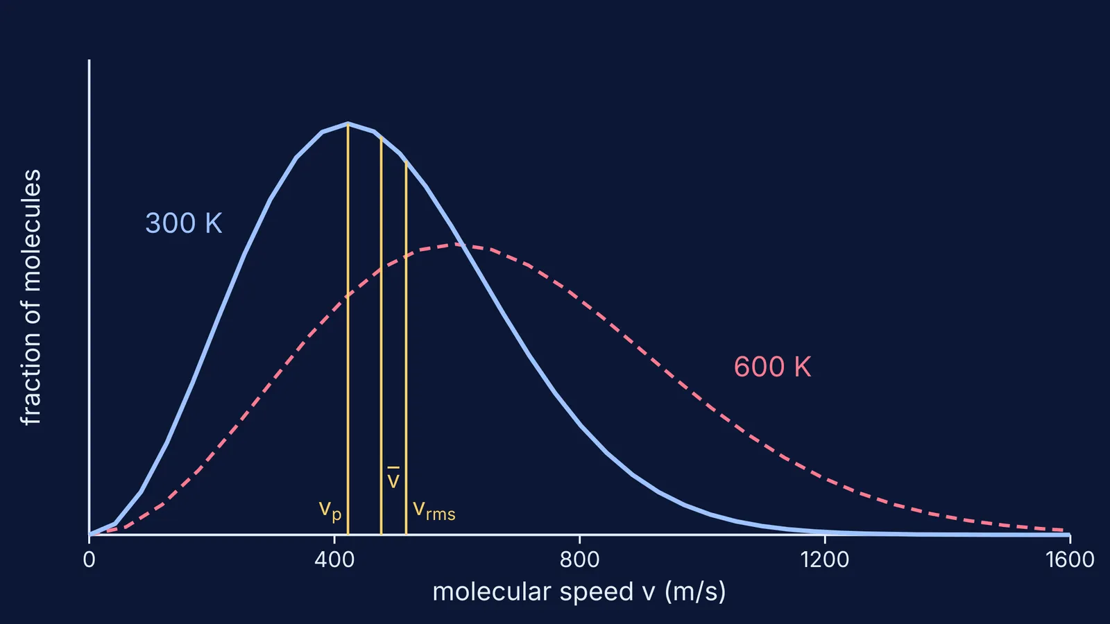
Two factors fight each other. The v² term grows with speed, because there are more ways (more directions in 3D) to move at a larger speed. The exponential term shrinks fast, because high kinetic energy is rare. The result is a lopsided hump:
It starts at zero: almost no molecule is perfectly still.
It rises to a peak at the most probable speed.
It falls away in a long tail on the high-speed side.
Heat the gas and the peak moves right and gets lower, while the total area (all the molecules) stays the same.
How are most probable, mean and rms speeds different?
All three come straight out of Maxwell's curve, with R the gas constant and M the molar mass in kg/mol (formulas):
Most probable speed, the peak of the curve: v_p = √(2RT/M).
Mean speed, the ordinary average: v̄ = √(8RT/πM).
Root-mean-square speed, the square root of the average of v²: v_rms = √(3RT/M).
Because 2 < 8/π (about 2.55) < 3, the order never changes: v_p < v̄ < v_rms. Divide through and you get the ratio 1 : 1.128 : 1.225, the same for every ideal gas at every temperature.
Because kinetic energy depends on v², the rms speed is the one tied directly to temperature and pressure. That is also why, at a fixed temperature, rms speed does not change with pressure, and why the speed of sound in a gas is a fixed fraction of the rms speed for a given gas.
Worked example: how fast is nitrogen at room temperature?
Take nitrogen (N₂) at 300 K. Use R = 8.314 J mol⁻¹ K⁻¹ (NIST value) and M = 0.028 kg/mol.
Work out RT/M once: 8.314 × 300 / 0.028 ≈ 89,100 m²/s².
Most probable speed: √(2 × 89,100) ≈ 422 m/s.
Mean speed: √(2.546 × 89,100) ≈ 476 m/s.
Rms speed: √(3 × 89,100) ≈ 517 m/s.
Now double the temperature to 600 K. Every speed rises by √2, not by 2: about 597, 674 and 731 m/s.
The first answer matches the 422 m/s quoted for N₂ at 300 K in the reference article on the distribution. Before you submit, check:
Is M in kg/mol, not g/mol? Forgetting this makes your answer about 31.6 times too large (√1000).
Is T in kelvin, not °C?
Did the question ask for the most probable, mean or rms speed?
If T changes, did you scale by the square root?
Is your answer a few hundred m/s? If not, recheck the units.
If the shift of the curve with temperature still feels abstract, the Fermi Simulation Lab has interactive simulations for ideas that are easier to see than to read. For more numericals like the one above, the Fermi Problem Library has worked problems with a step-by-step solver that explains the reasoning rather than printing an answer.
Maxwell's curiosity ranged well beyond gases. Read about James Clerk Maxwell and the first colour photograph of 1861.