
On this page
In late 1967, physicists from MIT and the Stanford Linear Accelerator Center (SLAC) fired electrons at liquid hydrogen and counted how they bounced. By spring 1968 the numbers suggested that the proton was not a soft, smooth blob: electrons seemed to be hitting something small and hard inside it. Those hard grains were later identified as up and down quarks, and the experiments' leaders, Jerome Friedman, Henry Kendall and Richard Taylor, shared the 1990 Nobel Prize in Physics, as Physics Today reported.
What did Friedman, Kendall and Taylor set out to measure?
By the early 1960s, Robert Hofstadter's electron experiments at Stanford had shown that protons and neutrons are about 10⁻¹³ cm across, but most physicists thought of them as soft objects with a fuzzy inside, according to Michael Riordan's SLAC history of the discovery. (See how Robert Hofstadter measured the size of a proton.) In 1964, Gell-Mann and Zweig had proposed quarks inside protons and neutrons, with charges of 1/3 or 2/3 of the electron's charge, but no search found a fractionally charged particle, so most physicists treated quarks as handy maths, not real objects.
SLAC's new tool was a two-mile-long linear accelerator. Taylor's Lindau Nobel research profile says it was planned to reach energies around 22 GeV, and scattering runs began in 1967. The earlier elastic run, at up to 20 GeV, was generally read as a sign of a soft proton with no hard core (Riordan, SLAC).
What is deep inelastic scattering?
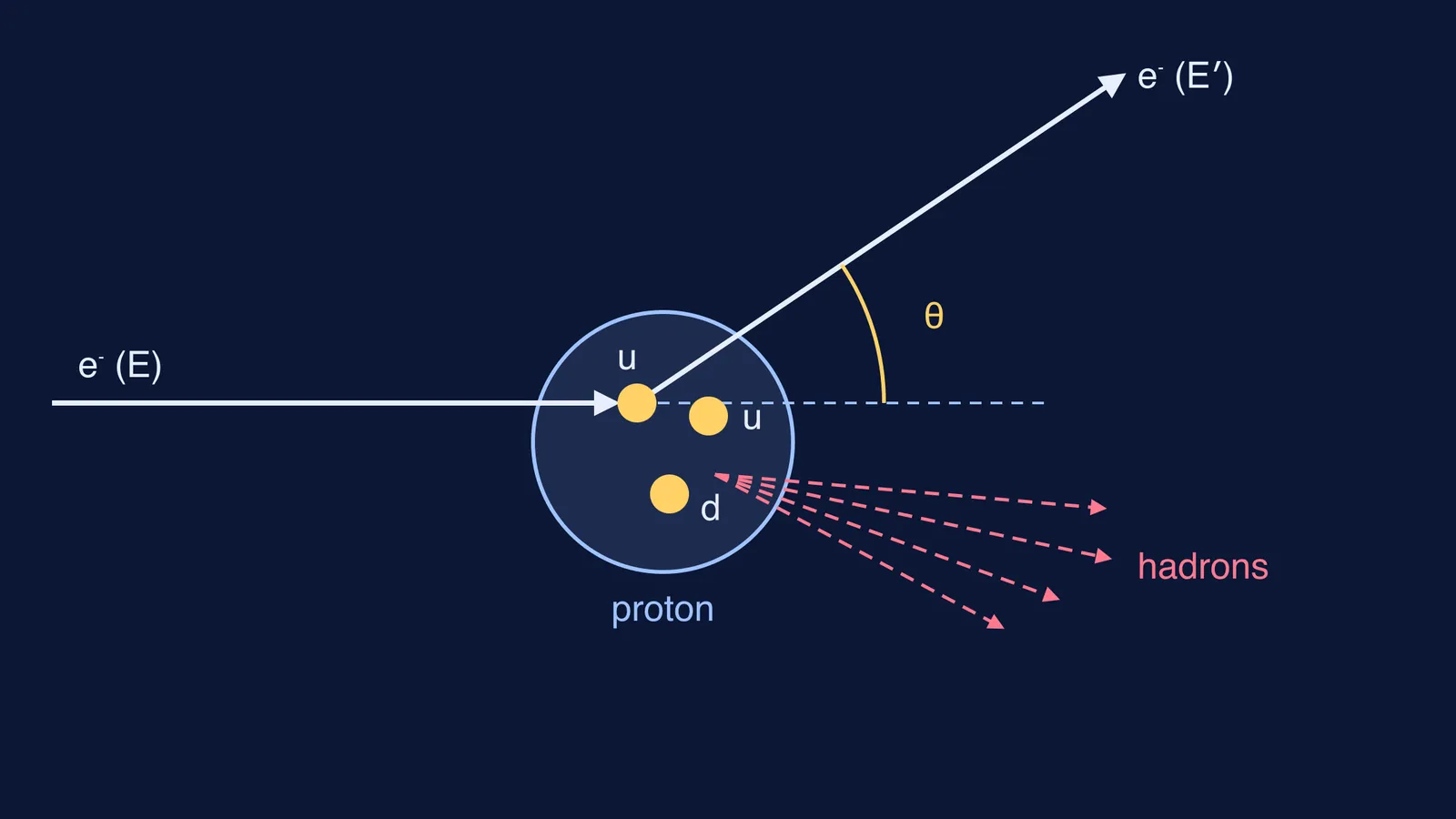
Deep inelastic scattering is a collision in which the electron gives so much energy to the proton that the proton breaks apart, and the electron bounces away with much less energy (Riordan, SLAC).
Spectrometers in SLAC's End Station A, built largely under Taylor's direction, picked out electrons bouncing off at a chosen angle and measured their energy. In the first inelastic run, at 6 degrees, the counts were much higher than expected. Electrons give off photons as they scatter, and removing these radiative effects from the raw data took months. By spring 1968 it was clear they did not explain the high rate: deep inelastic scattering fell much more slowly with momentum transfer than elastic scattering did, as if the electrons were hitting a hard core. Riordan likens it to Rutherford's gold-foil surprise; try that in our Rutherford gold foil simulation guide.
Why did the SLAC results point to quarks?
One surprising graph was not enough; rival explanations had to be ruled out. Each step below comes from Riordan's account:
Scaling (April 1968). On James Bjorken's suggestion, Kendall plotted the data against one combined variable, and cross sections measured at different energies fell on a single curve.
Partons (August 1968). Richard Feynman explained the curve with pointlike constituents he called partons. His x is the fraction of the proton's momentum carried by the struck parton.
Spin (1969). Larger-angle data, shown in summer 1969, fitted charged partons with spin 1/2, as quarks should have.
Neutrons versus protons (1970 to 1973). The neutron-to-proton ratio fell from about 1 at low x to about 0.3 at high x, ruling out models that needed 1 everywhere.
Gluons. Some sum rules came out about a factor of 2 too small for a simple three-quark proton, unless neutral gluons carried about half the proton's momentum.
The first 6° and 10° results appeared in two Physical Review Letters papers in October 1969: Bloom and colleagues and Breidenbach and colleagues.
Worked example: what fraction of the proton did the electron hit?
These numbers are illustrative, not from the papers; the formulas come from Riordan's account, and 18° was one of the team's angles. An electron of energy E = 10 GeV comes out at θ = 18° with E′ = 4 GeV. The proton's mass is 0.938 GeV (NIST CODATA).
Energy lost: ν = E − E′ = 6 GeV.
Momentum transfer: Q² = 2EE′(1 − cos θ) = 2 × 10 × 4 × (1 − 0.951) ≈ 3.92 GeV².
Feynman's variable: x = Q²/(2Mν) = 3.92/(2 × 0.938 × 6) ≈ 0.35.
So the struck parton carried about 35% of the proton's momentum.
Now check the 2/3 prediction. The hit rate goes with charge squared, so with only three quarks sharing momentum the same way, proton (uud) gives (2/3)² + (2/3)² + (1/3)² = 1 and neutron (udd) gives (2/3)² + (1/3)² + (1/3)² = 2/3. The real ratio did not stay at 2/3: it neared 1 at low x, where quark-antiquark pairs dominate, and fell to about 0.3 at high x.
What can you learn from how they worked?
Rule out the boring explanation first, as the months of corrections did.
Plot in the variable theory suggests; scaling appeared on Kendall's new axis.
Design a test that separates models, like the neutron comparison.
If scattering angles are hard to picture, the Fermi Simulation Lab has interactive simulations for ideas that are easier to see than to read. For practice, the Fermi Problem Library has worked problems with a step-by-step solver that explains the reasoning.
Try the worked example again with θ = 26° and the same E and E′, and see how x changes.