
On this page
In May 1964, Arno Penzias and Robert Wilson at Bell Laboratories in New Jersey got an answer that made no sense. Their antenna, listening at a wavelength of 7.35 cm, read several kelvin warmer than expected, wherever they pointed it. That stubborn hiss was the cosmic microwave background (CMB), radiation that Wilson's 1978 Nobel lecture describes as "considered a relic of the explosion at the beginning of the universe".
What did Penzias and Wilson actually hear?
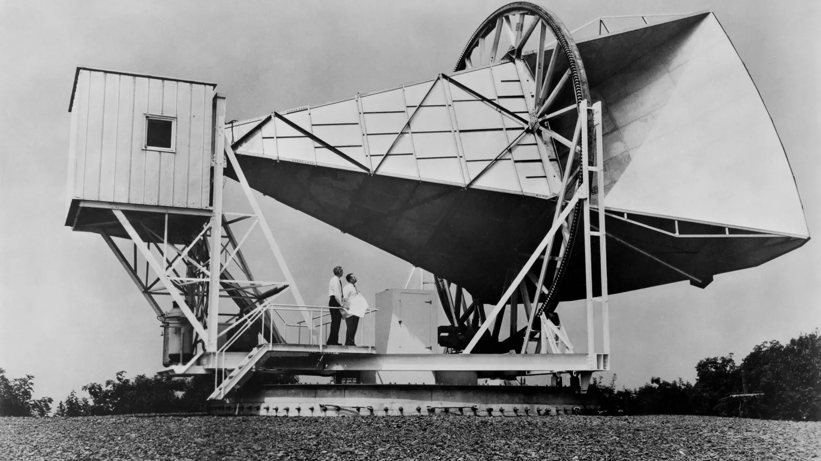
Their instrument was a 20-foot horn-reflector built by A. B. Crawford's team in 1960 to receive signals bounced off the Echo satellite, according to Wilson's Nobel lecture. Its horn shape shielded the receiver from the warm ground. In 1963 the two began turning it into a radio telescope with a 7.35 cm maser amplifier. In radio astronomy, noise is quoted as a temperature: that of a resistor delivering the same noise power.
Their first task was meant to be a dull check: earlier low-frequency measurements put our galaxy's halo below 0.1 K at 7 cm, so the sky away from the Milky Way should have read almost nothing. Their first record, dated 20 May 1964, showed the antenna at about 7.5 K, against an expected 3.3 K: 2.3 K from the atmosphere plus 1 K from the antenna walls and the ground.
How did they rule out pigeons, New York and the bomb?
They listed every suspect and tested each one, as Wilson recounts in the lecture:
The atmosphere: their own sky scans fitted the standard value, not the doubled one some astronomers suggested.
Man-made noise: pointing at New York City, or anywhere on the horizon, gave no more than the warm ground alone.
Our galaxy: extrapolations predicted only about 0.02 K from the coldest sky, and the excess did not follow the Milky Way.
The antenna: they evicted a pair of pigeons that had coated the horn with "a white material familiar to all city dwellers", and in spring 1965 taped over the riveted joints. Each step gave only a small reduction.
Time: after almost a year the excess had not changed, ruling out the solar system and the charged particles left in the Van Allen belts by a 1962 high-altitude nuclear explosion.
Who explained the cosmic microwave background?
Penzias mentioned the noise to Bernard Burke of MIT, who recalled work by P. J. E. Peebles in Robert Dicke's group at Princeton, Wilson writes in the lecture. Peebles had calculated that the universe should be filled with relic blackbody radiation at a minimum of 10 K, and Dicke, Roll and Wilkinson were setting up an experiment to find it.
The two groups published side by side in The Astrophysical Journal in July 1965: Princeton's theory letter, Cosmic Black-Body Radiation, and Bell Labs' A Measurement of Excess Antenna Temperature at 4080 Mc/s. Bell Labs' letter stayed out of cosmology and reported that the excess temperature was "within the limits of our observations, isotropic, unpolarized, and free of seasonal variations".
Roll and Wilkinson confirmed it in December 1965, measuring 3.0 ± 0.5 K at 3.2 cm. The 1978 Nobel Prize in Physics gave half to Penzias and Wilson "for their discovery of cosmic microwave background radiation"; the other half went to Pyotr Kapitsa for low-temperature physics.
The modern value of the CMB temperature is 2.72548 ± 0.00057 K, from D. J. Fixsen's 2009 review of the measurements. Read on: how COBE found the Big Bang's glow and its ripples, how Lummer and Pringsheim measured the blackbody spectrum, and how hot gas shifts the glow in the Sunyaev-Zeldovich effect.
How can you work a puzzle the way Penzias and Wilson did?
Their real tool was a noise budget: add up everything you know, subtract it from what you measure, and see what is left. Here are the numbers for the original antenna from the results table in Wilson's lecture:
Measured antenna temperature: 6.7 ± 0.3 K.
Atmosphere: 2.3 ± 0.3 K.
Waveguide and antenna loss: 0.9 ± 0.3 K.
Back lobes (pickup from the ground): 0.1 ± 0.1 K.
Known sources together: 3.3 ± 0.7 K, so the leftover is 6.7 − 3.3 = 3.4 K, quoted as 3.4 ± 1 K.
Because these errors were not statistical, they added the largest possible error from each source. Even that worst case, 1 K, was much smaller than the 3.4 K left over.
Use the same steps when a practical reading looks wrong:
Write down what you expected, as a sum of parts.
List every suspect, including boring ones like loose joints or a warm room.
Test one suspect at a time and note how much each fix changed the reading.
Repeat on another day. A fault drifts; a real effect stays put.
If a numerical like this leaves you unsure which step went wrong, the Fermi Problem Library has a step-by-step solver that explains the reasoning. For ideas easier to see than to read, try the Fermi Simulation Lab.
Next time a result refuses to behave, run the budget before you blame the instrument.