On this page
Why could standard X-rays not show cross-sectional slices?
Conventional radiography has a fundamental physical limitation: it produces a 2D shadow of a 3D body. Every anatomical layer along the beam path—skin, muscle, bone, and organs—superimposes onto a single film, flattening depth, as explained in our guide on how ordinary X-rays produce shadow images of bones. High-density bones cast broad shadows that mask subtle soft-tissue tumors.
In 1956, South African physicist Allan Cormack confronted this problem at Groote Schuur Hospital in Cape Town, as recorded in his Nobel biographical memoir. Hospital charts assumed patients were uniform cylinders of water. Cormack recognized that tissue variations distort absorption, an issue explored in Louis Harold Gray and the measurement of radiation dose. In his 1980 Nobel lecture in *Science*, Cormack showed that mapping attenuation coefficients beforehand turned imaging into an inverse problem in calculus.
How does a line integral measure tissue attenuation?
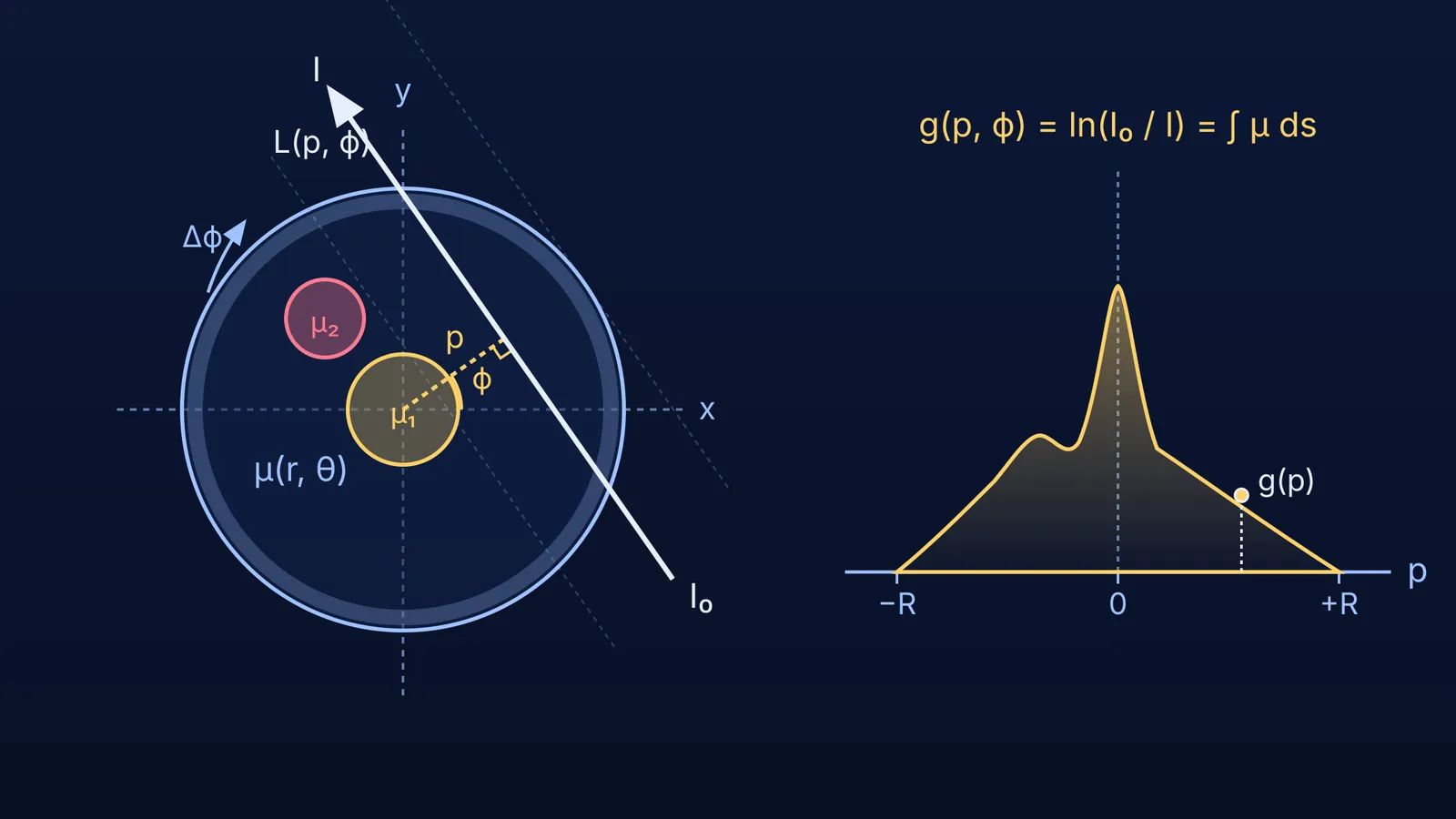
The physical link between transmitted radiation and tissue density is the Beer-Lambert law. As a narrow beam of monoenergetic radiation travels along a path L, its intensity drops across each infinitesimal element ds in proportion to the local linear attenuation coefficient μ(x, y):
dI = −μ(x, y) · I · ds
Integrating along path L yields the total attenuation:
ln(I₀ / I) = ∫_L μ(x, y) ds
An external detector measures incident intensity I₀ and transmitted intensity I, giving the value of the line integral. This process mirrors viewing a definite integral as the limit of a sum.
To organize the scan, Cormack parameterized each line by its perpendicular distance p from the origin and normal angle ϕ:
r · cos(θ − ϕ) = p
The measured profile g(p, ϕ) = ∫_L μ(r, θ) ds represents the projection of the slice at angle ϕ. In his 1963 paper in the *Journal of Applied Physics*, Cormack set out to invert this integral to find μ(r, θ).
How did Allan Cormack solve the reconstruction equations?
The core challenge was that a single line integral only yields a total sum along a path, not the point-by-point values. In 1917, Johann Radon had proved mathematically that a 2D function can be reconstructed from its line integrals, though his work remained unknown in medicine. In 1956, Ronald N. Bracewell independently developed projection reconstruction for solar maps in the *Australian Journal of Physics*.
In his 1963 mathematical paper, Cormack formulated a series expansion method. He expanded the unknown attenuation μ(r, θ) in polar angle θ using a Fourier series:
μ(r, θ) = Σ μ_n(r) · exp(i · n · θ)
He expanded projection data g(p, ϕ) similarly in angle ϕ:
g(p, ϕ) = Σ g_n(p) · exp(i · n · ϕ)
Substituting these series into the line integral equation decoupled the angular dependence, reducing the 2D problem into independent 1D Abel integral equations for each radial component μ_n(r). Cormack solved these using orthogonal expansions with Chebyshev and Zernike polynomials, yielding an analytical inversion formula.
Worked example: why is a single projection not enough?
Consider a 2 × 2 grid of unknown tissue values [a, b; c, d] to see why multiple angles are essential:
Horizontal rays (0°):
Beams produce row sums a + b = 7 and c + d = 11, leaving infinite combinations for individual cells.
Vertical rays (90°):
Beams produce column sums a + c = 6 and b + d = 12. These equations share a redundant degree of freedom because 7 + 11 = 6 + 12 = 18.
Diagonal ray (45°):
A diagonal sum a + d = 9 breaks the ambiguity, resolving the system uniquely: a = 2, b = 5, c = 4, and d = 7.
In human anatomy, smooth tissue distributions replace discrete cells. Cormack showed that measuring continuous line integrals across angles from 0 to π collects enough independent equations to determine μ(r, θ) uniquely.
How was Cormack's mathematical model tested experimentally?
After moving to Tufts University, Cormack built an experimental scanner and published experimental proof in the *Journal of Applied Physics* in 1964. He designed a test phantom simulating a head cross-section:
An outer aluminum ring with a 20 cm diameter modeled the skull.
The interior was filled with Lucite to model soft brain tissue.
Aluminum cylinders simulated tumors.
To avoid polychromatic beam hardening, Cormack used a Cobalt-60 source emitting gamma rays at 1.17 and 1.33 MeV, detected by a collimated Geiger counter. Measuring along 19 lines across 25 angles (at 7.5° intervals) yielded 475 transmission values. Using computer code, he successfully reconstructed the attenuation values.
His work went unnoticed until Godfrey Hounsfield independently built the first clinical scanner at EMI, reported in *The British Journal of Radiology* in 1973. Cormack and Hounsfield shared the 1979 Nobel Prize in Physiology or Medicine, as recorded in the Nobel Assembly press release.
What does Cormack's method teach STEM students today?
Cormack's work illustrates how pure mathematics transforms applied medical science.
When studying integration, coordinate transformations, and wave physics, connecting equations to physical devices makes mathematical principles memorable. The Fermi Concept Library organizes every concept in physics, chemistry, biology, mathematics and computing, each with its own lesson and its place in the map. When practicing problem sets, the Fermi Problem Library provides worked problems with a step-by-step solver that explains the reasoning rather than printing an answer. For principles that are easier to see than to read—such as coordinate rotations and beam attenuation—the Fermi Simulation Lab offers interactive simulations for ideas that are easier to see than to read.