On this page
In Young's double-slit experiment (YDSE), two coherent beams superpose on a screen to produce alternating bright and dark fringes of uniform width. A classic question in school board exams, JEE Main, and NEET-UG asks what happens if you cover one of the two slits with an opaque card.
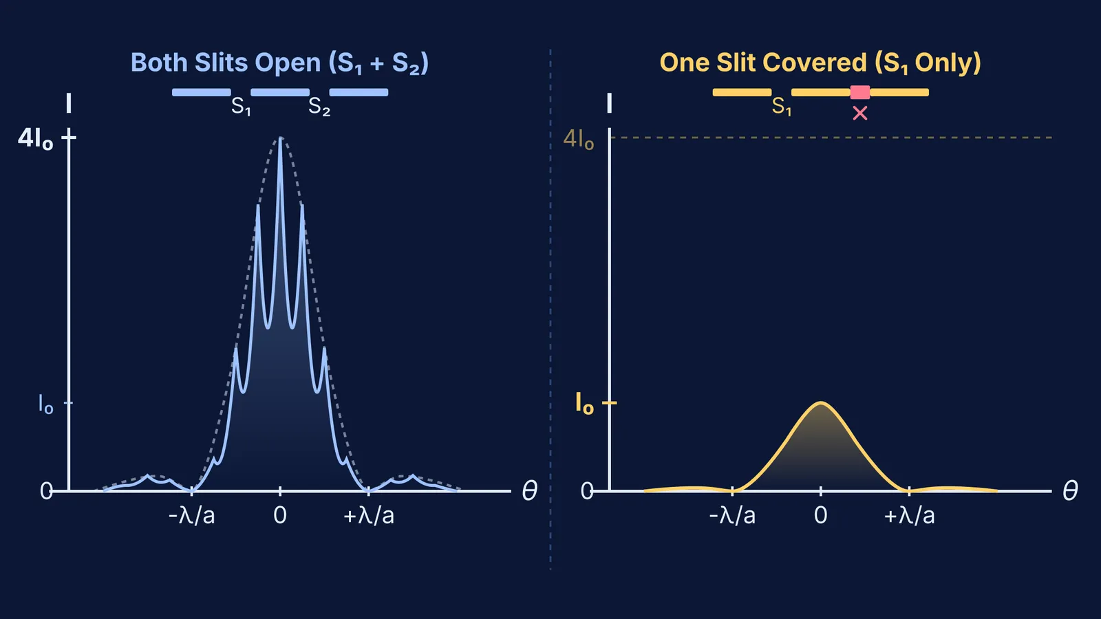
The interference fringes completely vanish. Instead of a series of closely spaced, high-contrast bands, you observe a single-slit diffraction pattern: a broad central maximum flanked by faint secondary bands. Furthermore, the peak intensity at the centre drops to exactly one-fourth of the two-slit maximum.
What happens to the interference fringes when one slit is covered?
Interference requires two mutually coherent wave trains arriving at the screen with a stable phase relationship. In his landmark 1804 Bakerian Lecture, Thomas Young placed a narrow card into a sunlight beam and intercepted light on one side with a screen. Young observed that the moment one path was blocked, every interior interference fringe immediately disappeared.
When both slits are open, destructive interference drives intensity at the dark fringes to zero because crests from one slit coincide with troughs from the other. Covering one slit stops this cancellation. Light from the open slit reaches those formerly dark regions unimpeded. Understanding the difference between interference and diffraction makes it clear why sharp fringes give way to a smooth single-slit envelope.
Why does the central peak intensity drop to one-fourth?
If each slit transmits an electric field of amplitude E₀, the intensity from one slit alone is proportional to E₀², denoted as I₀.
When both identical slits are open, waves reach the central point with zero path difference. Their electric fields add constructively to E_total = 2E₀. Because intensity is proportional to amplitude squared, the central bright fringe reaches a peak of I_max ∝ (2E₀)² = 4I₀, as shown in OpenStax University Physics Volume 3.
Covering one slit leaves only one wave of amplitude E₀. Peak intensity drops from 4I₀ to I₀, a 75% reduction that leaves 25% of the original peak brightness.
For addressing concept gaps across wave optics, the Fermi Concept Library covers every concept in physics, chemistry, biology, mathematics and computing, each with its own lesson and its place in the map.
How does single-slit diffraction differ from double-slit interference?
Covering one slit alters the spatial geometry of the light distribution:
Fringe width: In double-slit interference, all fringes share equal linear width β = λD / d, where d is slit separation and D is screen distance.
Central maximum width: In single-slit diffraction, the central maximum is bounded by first minima at a sin θ = ±λ, giving a linear width of W = 2λD / a. This central peak is 2d / a times wider than an individual double-slit fringe.
Intensity fall-off: Double-slit fringes maintain high contrast across the central region. In single-slit diffraction, secondary peaks plunge to roughly 4.5% of I₀ (approximately 0.045 I₀, or 4.7% by exact calculation) for the first side peak and 1.6% for the second, as documented in single-slit diffraction intensity measurements.
As analysed in Max Born and Emil Wolf's *Principles of Optics*, the observed double-slit pattern is the product of single-slit diffraction and two-slit interference. Blocking one slit exposes the single-slit profile. You can also predict the single-slit pattern first by tracing how wavefronts spread around aperture edges.
What happens if the remaining slit is extremely narrow?
According to the NCERT textbook portal curriculum for Class 12 Physics, if an exam problem specifies that slit width a is comparable to or smaller than wavelength λ (a ≤ λ), the first diffraction minimum at sin θ = λ / a cannot exist on a screen.
In that limiting case, the central maximum spreads across all angles, producing faint, uniform illumination without visible minima. In real experiments where a is a fraction of a millimetre, a clear single-slit diffraction pattern is always observed. Keeping this distinction in mind prevents common wave optics traps in competitive exams.
How do you solve slit-covering numericals step by step?
As demonstrated in Thomas V. Marcella's aperture analysis in the *European Journal of Physics*, double-slit and single-slit distributions can be evaluated systematically. Consider a standard laboratory problem: slit separation d = 0.20 mm, slit width a = 0.04 mm, wavelength λ = 600 nm, and screen distance D = 1.0 m.
Double-slit fringe width: β = λD / d = (600 × 10⁻⁹ × 1.0) / (0.20 × 10⁻³) = 3.0 mm.
Single-slit central width: W = 2λD / a = 2(600 × 10⁻⁹ × 1.0) / (0.04 × 10⁻³) = 30.0 mm.
Width ratio and replaced fringes: The central maximum spans a width of W / β = 2d / a = 10 fringe widths. Before covering the slit, this central region contained 9 bright interference fringes (orders m = 0, ±1, ±2, ±3, and ±4, with the m = ±5 orders missing because they coincided with the diffraction zeros).
Intensity drop: Peak intensity falls by 75%, from 4I₀ to I₀.
Covering one slit replaces this multi-fringe pattern across the 30.0 mm central zone with a single continuous diffraction maximum at 25% of the original peak brightness.
For students tackling numericals on slit widths, path differences, and intensity ratios, the Fermi Problem Library provides worked problems with a step-by-step solver that explains the reasoning rather than printing an answer. To visualise wavefronts bending through slits in real time, explore the Fermi Simulation Lab, which features interactive simulations for ideas that are easier to see than to read.