

On this page
A single-slit simulation lets you test the formula you memorised: narrow the slit, widen it or change the wavelength, and check whether the bright band does what you said it would. The trick is to predict before you move anything.
What does a single-slit diffraction pattern look like?
Light through one narrow slit lands on the screen as a wide, bright central band with much fainter bands either side. OpenStax's University Physics Volume 3 describes the central maximum as larger than the maxima on either side, with intensity falling off rapidly.
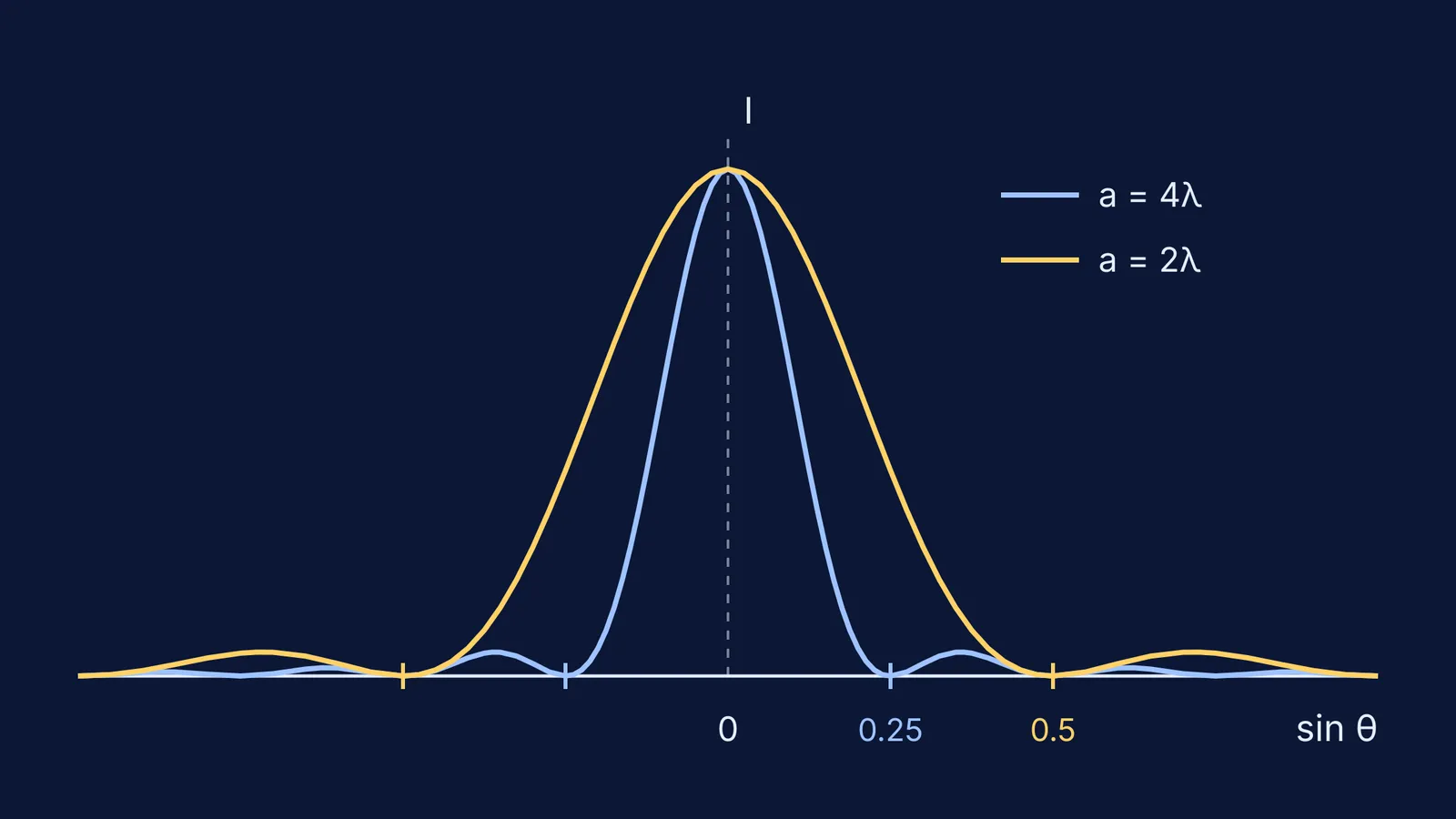
The fall-off is steep. The intensity follows I = I₀(sin β / β)², where β = πa sin θ / λ, and the first side maximum is only about 0.045 I₀, or 4.5% of the centre, according to OpenStax's section on single-slit intensity. The second is about 1.6%, so in a simulation the side bands can look almost invisible.
Where do the first minima fall in single-slit diffraction?
Dark fringes fall where a sin θ = mλ, for m = ±1, ±2, ±3 and so on, where a is the slit width and λ is the wavelength (OpenStax, section 4.1). Notice that m = 0 is not on the list. Straight ahead, waves from every part of the slit arrive in phase, so the centre is bright.
The first minima therefore sit at sin θ = ±λ/a. On a screen a distance D away, and for small angles, the distance from the centre to the m-th minimum is y = mλD/a, the relation HyperPhysics uses in its single-slit calculator.
OpenStax's worked example is a good check of your own arithmetic: 550 nm light through a 2.00 μm slit puts the first minimum at 16.0° and the second at 33.4°.
One edge case catches students: if the slit is narrower than the wavelength, λ/a is bigger than 1, no angle has a sine that large, and there are no minima at all.
How does slit width change the central maximum?
The central maximum runs from the first minimum on one side to the first minimum on the other. For small angles, which means a slit much wider than the wavelength, its angular width is about 2λ/a (OpenStax, section 4.2), which on the screen is 2λD/a. Slit width sits in the denominator. Narrow the slit and the pattern spreads out. Widen it and the pattern shrinks towards a sharp spot.
Worked example
Take a slit width a = 0.10 mm, wavelength λ = 600 nm and a screen D = 1.0 m away.
First minimum: y₁ = λD/a = (600 × 10⁻⁹ × 1.0) / (1.0 × 10⁻⁴) = 6.0 × 10⁻³ m, so 6.0 mm from the centre.
Central maximum width: 2 × 6.0 mm = 12 mm.
Halve the slit to 0.05 mm: the central maximum doubles to 24 mm.
Double the slit to 0.20 mm: it halves to 6 mm.
Keep a = 0.10 mm but move the screen to 2.0 m: 24 mm again, because y grows with D.
Each side maximum is about λD/a wide, half the central band. That factor of two is a common exam trap.
How does wavelength change the diffraction pattern?
Wavelength sits in the numerator of y = mλD/a, so the whole pattern scales with it. Keep a = 0.10 mm and D = 1.0 m from the example and switch from 600 nm to 450 nm light. The first minimum moves in from 6.0 mm to 4.5 mm, and the central band shrinks from 12 mm to 9 mm. Longer wavelengths spread more through the same slit.
What really sets the pattern is the ratio λ/a. Double both the wavelength and the slit width and nothing on the screen moves.
How should you use a single-slit diffraction simulation?
Use this predict-then-test plan:
Write down a, λ and D, and calculate y₁ = λD/a.
Predict the central maximum width (2y₁), and say aloud what halving a should do.
Move one slider only. Measure from the centre to the first dark band, not to where the glow fades.
Compare. If you are out by a factor of two, you probably mixed up the full width and the half-width.
Push to the edge: make a smaller than λ and check that the minima disappear.
Change λ and a by the same factor and confirm that the pattern stays put.
The Fermi Simulation Lab has interactive simulations for ideas that are easier to see than to read, and the same habit works there. If the numbers trip you up, the Fermi Problem Library has worked problems with a step-by-step solver that explains the reasoning rather than printing an answer.
For exam-style practice on these formulas, work through our single-slit diffraction and Malus's law problems. To see how one slit differs from two, read Young's double-slit fringe width problems and traps, and for more slider experiments, try learning waves with simulations.


