On this page
In the Class 11 viscosity practical you drop steel balls down a tube of glycerine, time them between rubber bands and read the viscosity off a graph. Three things decide how close you get: the timing marks, the slope, and the tube walls, which push your answer too high.
How do you find the coefficient of viscosity from terminal velocity?
A falling ball speeds up until its weight is balanced by buoyancy plus the viscous drag 6πηrv; after that it falls at a constant terminal velocity v (NCERT Laboratory Manual, Experiment 13).
That balance gives v = 2r²(σ − ρ)g / 9η, where r is the ball's radius, σ the density of steel and ρ that of the liquid. So a graph of v against r² is a straight line through the origin, and η = 2(σ − ρ)g / (9 × slope). With the slope in m⁻¹ s⁻¹, η comes out in N s m⁻² (Pa s).
How do you set up the tube and the timing marks?
The NCERT procedure, in short:
Note the room temperature and your stopwatch's least count.
Fill a tube about 1.25 m long and 4 cm across with glycerine, free of air bubbles.
Put rubber bands A, B and C on it with AB = BC, about 30 cm each, and A about 40 cm below the mouth so the ball reaches terminal velocity first.
Use steel balls 1.0 mm to 3 mm across, rinsed in glycerine so they carry no bubbles.
Drop each ball through a short inlet tube so it falls along the axis.
Start two stopwatches at A; stop one at B (t₁) and the other at C (t₂).
Temperature matters: a KVIS physics note lists glycerin at 12 N s m⁻² at 0 °C but 0.27 N s m⁻² at 30 °C (Stokes' law and laminar flow, KVIS). A value without a temperature means little.
Worked example: from stopwatch times to η
These readings are made up for practice and built so the true viscosity is 1.00 Pa s. They use σ = 7810 kg m⁻³ for chrome steel (Carter Bearings, bearing materials), ρ = 1261 kg m⁻³ for glycerol at 20 °C (PubChem, glycerol density), g = 9.8 m s⁻², h = 30 cm and a 4 cm tube.
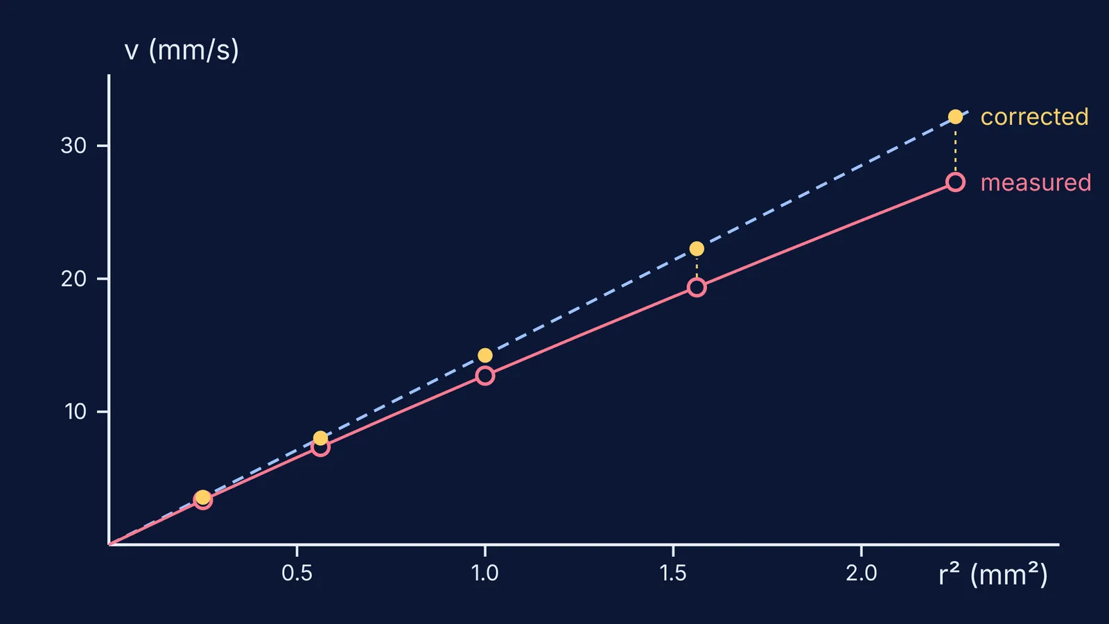
1.0 mm ball: t = 89.2 s, v = 3.36 mm/s, v/r² = 13.45
1.5 mm ball: t = 40.8 s, v = 7.35 mm/s, v/r² = 13.07
2.0 mm ball: t = 23.6 s (and 47.2 s to C), v = 12.71 mm/s, v/r² = 12.71
2.5 mm ball: t = 15.5 s, v = 19.35 mm/s, v/r² = 12.39
3.0 mm ball: t = 11.0 s, v = 27.27 mm/s, v/r² = 12.12
Using the end points, slope = (27.27 − 3.36) / (2.25 − 0.25) = 11.95 mm s⁻¹ per mm², or 1.195 × 10⁴ m⁻¹ s⁻¹. Then η = 2 × 6549 × 9.8 / (9 × 11 950) = 1.19 Pa s, about 19% too high. The v/r² column shows why: it should be constant, but it falls as the balls get bigger.
Why does the wall effect make your viscosity too high?
Liquid pushed aside by the ball must squeeze through the gap between ball and tube, which adds drag. Researchers at IIT Kanpur note that putting a narrow-tube speed into Stokes' formula gives an apparent viscosity larger than the true one, a deviation driven by the Reynolds number and the ball-to-tube radius ratio (Singh, Sharma and Gupta-Bhaya, arXiv).
A first-order wall correction is v∞ = v(1 + 2.4r/R), where R is the tube's inner radius (KVIS note on wall effects). In a 4 cm tube the factor is 1.06 for the 1 mm ball but 1.18 for the 3 mm ball, so the big balls droop below the line.
Corrected, the v/r² values become 14.26, 14.25, 14.24, 14.25 and 14.30, the slope is 14.31 mm s⁻¹ per mm², and η = 1.00 Pa s. A screw gauge reading to 0.01 mm adds only 0.5% error in r on a 2 mm ball, so the wall, not your instrument, is the biggest error here.
If the correction step trips you up, the Fermi Problem Library has worked problems with a step-by-step solver that explains the reasoning rather than printing an answer.
What should you write under precautions and sources of error?
Wall effect: the walls add drag that grows with r/R; state the correction you applied.
Temperature: record it before and after.
Terminal velocity not reached: confirm t₂ = 2t₁.
Air bubbles, or balls that drift off the axis or touch the wall.
Parallax at the bands: keep your eye level with each one.
Reaction time: the 3 mm ball takes only 11 s, so repeat it more often.
Next, put error bars on your graph and find the uncertainty in the gradient, try the terminal velocity and viscosity simulation, or compare terminal velocity with linear vs quadratic drag. If Stokes' law feels shaky, start with its lesson in the Fermi Concept Library.