

On this page
When an object falls through a fluid like air or water, it does not accelerate indefinitely. Fluid resistance, or drag, pushes back against gravity. As the object speeds up, the drag force increases until it exactly balances the object's downward weight. At this point, the net force on the object becomes identically zero, and it continues falling at a steady, constant speed called terminal velocity. However, the exact mathematical model for this drag force depends heavily on the object's size, its geometric shape, and its speed through the medium. In university physics and classical mechanics, we typically model fluid drag as being proportional either to the velocity (linear drag) or to the square of the velocity (quadratic drag).
How does linear drag (Stokes' law) affect small particles?
Linear drag occurs when an object is very small or moves at very low speeds through a viscous fluid. This is known as a low Reynolds number regime, where the fluid flow around the object remains completely smooth and laminar without shedding any turbulent wakes or vortices.
In this regime, the drag force is directly proportional to the velocity: F_d = −bv. For a perfect sphere falling through a fluid, the proportionality constant b is given by Stokes' law as 6πrη, where r is the radius of the sphere and η is the dynamic viscosity of the fluid. Because the drag force required to perfectly balance the object's weight (mg) is simply bv, we can find the terminal velocity by setting mg = bv, which gives v_t = mg/b.
Microorganisms, fine dust particles, and pollen grains fall precisely into this category. For microscopic bacteria, the terminal velocity is extremely low, at just 2 μm/s, according to OpenStax University Physics.
How does quadratic drag affect falling skydivers?
For larger objects moving at much higher speeds through less dense fluids—like baseballs moving through air—the fluid flow separates from the object and becomes highly turbulent. This high Reynolds number regime is governed by quadratic drag.
Here, the drag force is proportional to the square of the velocity: F_d = −cv². The constant c is defined as ½CρA, where C is the dimensionless drag coefficient, ρ is the fluid density, and A is the object's cross-sectional area. Setting this drag force equal to the object's weight (mg = cv²) gives a terminal velocity of v_t = √(mg/c), which is equivalent to √((2mg)/(ρCA)).
This is the model that applies to everyday objects, from falling humans to hailstones. According to OpenStax University Physics, a 75-kg skydiver reaches a terminal velocity of approximately 98 m/s (350 km/h) falling head-first, while an 85-kg skydiver reaches only 44 m/s in a spread-eagle position, because spreading out significantly increases the cross-sectional area A.
If you find these transitions hard to picture, you can explore interactive models for such concepts in the Fermi Simulation Lab.
What are the equations of motion over time?
Finding exactly how the object's velocity changes over time requires solving the differential equation of motion. If you want to see the general rules for setting up these specific integrals, see our guide to Acceleration given as a function of v or x.
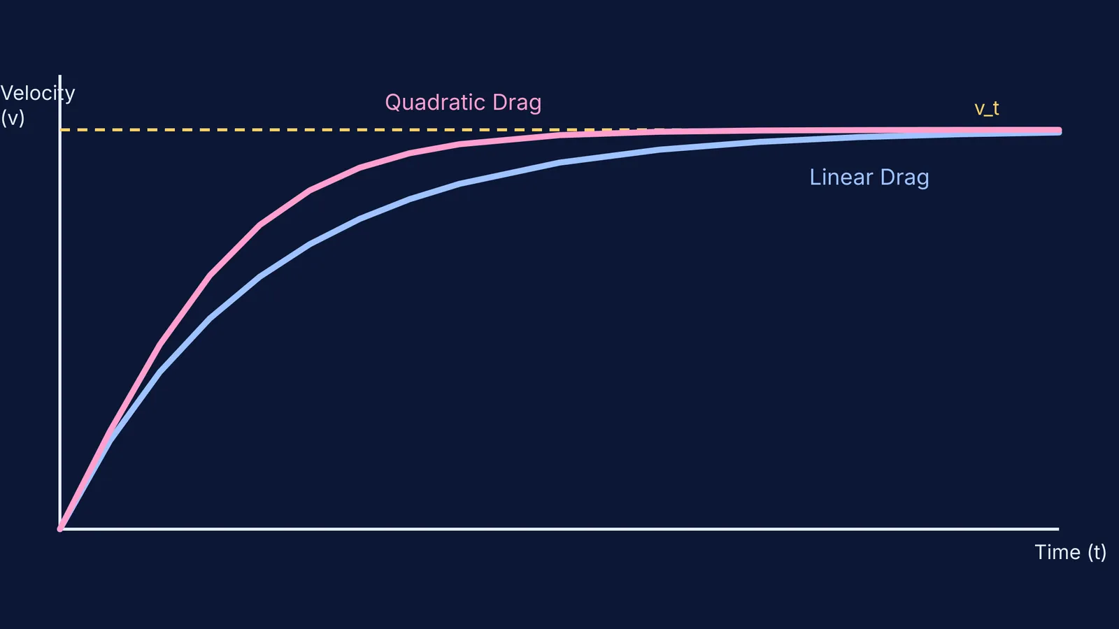
For linear drag, the equation of motion from Newton's second law is m(dv/dt) = mg − bv. Integrating this differential equation from an initial velocity of zero gives an exponential approach to terminal velocity:
v(t) = v_t (1 − e^(−bt/m))
For quadratic drag, the equation of motion is m(dv/dt) = mg − cv². The integral is slightly more complex, involving partial fractions, and it yields a hyperbolic tangent curve:
v(t) = v_t tanh(gt/v_t)
If you plot both of these velocity curves for two objects that happen to share the exact same terminal velocity, you will see that the object experiencing quadratic drag gains speed much faster initially. Because v² is smaller than v at low speeds (when expressed as a fraction of v_t), quadratic drag offers less resistance early in the fall, allowing the object to accelerate closer to the true rate of gravity for a longer time. If you ever forget which model applies to which geometric shape, the Fermi Concept Library maps out the complete derivations for both regimes. Both models are idealised approximations, but they provide the mathematical foundations for everything from settling dust to the Equation of trajectory of a projectile in real air.


