
On this page
Class 12 colligative properties questions often show two curves and one horizontal line and ask for the elevation in boiling point. They are easy once you know which gap to measure. Here is why the solution's curve sits lower, how to read ΔTb off the graph, and a worked example with real data for water.
How do vapour pressure curves show boiling point elevation?
Start with the definition. OpenStax Chemistry 2e puts it this way: "The boiling point of a liquid is the temperature at which its vapor pressure is equal to ambient atmospheric pressure."
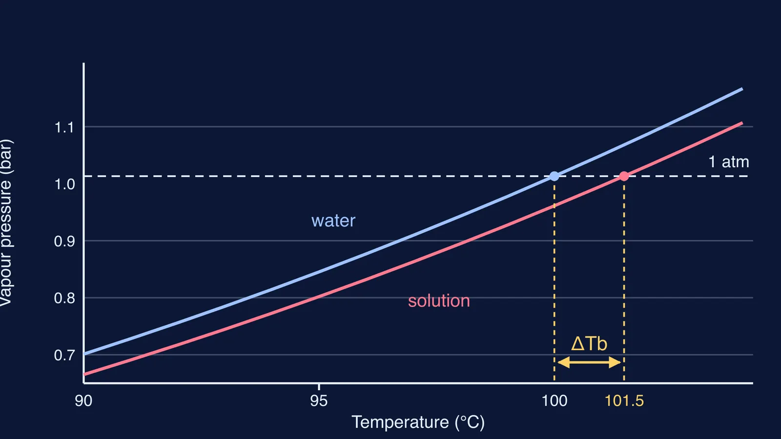
Dissolve a non-volatile solute, such as glucose, and fewer solvent molecules sit at the surface to escape, so the vapour pressure is lower at every temperature. In the OpenStax phase diagram, the liquid-vapour curve for the solution sits beneath the curve for the pure solvent.
Now draw a horizontal line at the outside pressure. At sea level that is 1 atm, which is 1.01325 bar, according to the NIST Guide to the SI. Both curves rise with temperature. The solvent's curve reaches the line first; the solution's starts lower, so it meets the line further right, at a higher temperature. The distance between those two crossing points along the temperature axis is the boiling point elevation, ΔTb.
How do you read ΔTb off the graph?
Use the same four steps every time:
Find the external pressure on the y-axis (1 atm unless the question says otherwise) and draw a horizontal line across.
Mark where the pure solvent's curve meets that line. Drop a vertical line to the x-axis and read Tb.
Do the same for the solution's curve and read the new boiling point, Tb′.
Subtract: ΔTb = Tb′ − Tb. For a non-volatile solute it is always positive.
Worked example: water and a 3 mol/kg solution
We drew the hero diagram from real data. The NIST Chemistry WebBook gives Antoine constants for water between 344 K and 373 K (A = 5.08354, B = 1663.125, C = −45.622, with P in bar and T in kelvin). Put in 100 °C and you get 1.013 bar, which is 1 atm, as expected.
Now dissolve 3 mol of a non-volatile non-electrolyte in 1 kg of water. One kilogram of water is about 55.5 mol (1000 g ÷ 18 g/mol), so the mole fraction of water is 55.5 ÷ 58.5 ≈ 0.949. For an ideal solution, Raoult's law says the solution's vapour pressure is 0.949 times the pure water value at every temperature.
At 100 °C the solution's vapour pressure is 0.949 × 1.013 ≈ 0.961 bar. That is below 1 atm, so the solution is not yet boiling.
Follow the lower curve to the right. It reaches 1.013 bar at about 101.5 °C.
So ΔTb ≈ 1.5 °C.
Check with the formula. OpenStax lists Kb for water as 0.512 °C/m, so ΔTb = Kb × m = 0.512 × 3 ≈ 1.54 °C. The graph (about 1.48 °C) and the formula agree to within about 0.05 °C; the formula is the dilute-solution shortcut for the same idea. Moving on to numericals? Our guide to boiling point elevation numericals using Kb and molality covers the unit traps.
You can also estimate it from slopes. Near 100 °C the solution's curve rises about 0.034 bar for every degree (from the same NIST constants). The vertical gap at 100 °C is 1.013 − 0.961 ≈ 0.052 bar. Divide: 0.052 ÷ 0.034 ≈ 1.5 °C. Because the curve is steep near boiling, a small vertical drop becomes only a small horizontal shift.
What mistakes do students make with these graphs?
Reading the vertical gap as ΔTb. The vertical gap is a pressure. ΔTb is a temperature, read along the x-axis.
Assuming the line is always 1 atm. On a mountain the outside pressure is lower, but the horizontal-gap rule still works. Our post on using the Clausius-Clapeyron equation to find water's boiling point in Shimla shows that calculation.
Letting the curves cross. For a non-volatile solute in an ideal solution, the lower curve is a fixed fraction of the upper one, so they never cross.
Forgetting about electrolytes. One mole of NaCl gives more particles than one mole of glucose, so its curve sits lower and its ΔTb is larger. Our guide to comparing i × m across solutions explains how to rank them.
How should you practise this before the exam?
Sketch the two curves from memory, draw the 1 atm line, and label Δp (vertical) and ΔTb (horizontal). Then solve one numerical both ways, from the graph and from Kb × m, and check they agree. If you are not sure why vapour pressure falls in the first place, the Fermi Concept Library covers each idea in chemistry in its own lesson. When a numerical goes wrong, the Fermi Problem Library has worked problems with a step-by-step solver that explains the reasoning rather than just giving an answer, so you can see which step went wrong.