On this page
Your equation, say x³ − x − 1 = 0, will not factorise, and the question only asks you to show a root exists between 1 and 2. That is the intermediate value theorem's job, and the proof takes a few lines once you know the two things to check.
What does the intermediate value theorem actually say?
OpenStax Calculus Volume 1 states it like this: if f is continuous over a closed, bounded interval [a, b] and z is any number between f(a) and f(b), then some c in [a, b] satisfies f(c) = z (OpenStax Calculus Volume 1, section 2.4).
For roots, take z = 0. If f is continuous on [a, b] and f(a) and f(b) have opposite signs, then 0 lies between them, so f(c) = 0 for some c between a and b. Picture an unbroken curve: to get from below the x-axis to above it, it has to cross.
The official JEE (Advanced) 2026 syllabus lists "intermediate value property of continuous functions" under Differential Calculus (JEE (Advanced) 2026 syllabus). The CBSE Class XII syllabus for 2026-27 lists continuity and differentiability but does not name the theorem (CBSE Mathematics (041) syllabus).
How do you show a root exists, step by step?
Move everything to one side: f(x) = 0.
Name the closed interval [a, b].
Prove f is continuous on all of [a, b], with a reason: a polynomial, a sum or product of continuous functions, or a quotient whose denominator is never zero there.
Compute f(a) and f(b) and show the signs differ.
Conclude: by the intermediate value theorem, there is c in (a, b) with f(c) = 0.
Step 3 is where marks leak: "f is continuous" with no reason is a claim, not a proof. For the rules, see our post on whether a continuous plus a discontinuous function is continuous, and continuity on a closed interval and the endpoint rule explains what "continuous on [a, b]" asks of the two ends.
Worked example: a standard "show that"
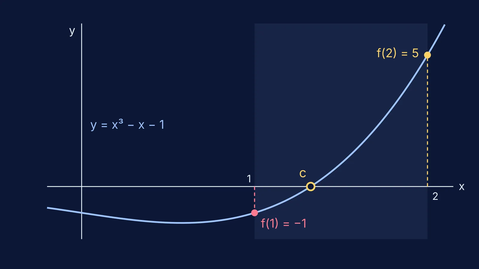
Show that x³ − x − 1 = 0 has a root between 1 and 2.
Let f(x) = x³ − x − 1. Since f is a polynomial, it is continuous on [1, 2]. Next, f(1) = −1 < 0 and f(2) = 5 > 0. Since f is continuous on [1, 2] and f(1) < 0 < f(2), the intermediate value theorem gives some c in (1, 2) with f(c) = 0.
To narrow it down, f(1.5) = 0.875 > 0, so the root lies in (1, 1.5). f(1.25) = −0.296875 < 0, so it lies in (1.25, 1.5). Each check halves the interval; this is the bisection method.
Exactly one root? The theorem only promises at least one. Here f′(x) = 3x² − 1 is at least 2 on [1, 2], so f is strictly increasing and crosses zero once. Uniqueness always needs an extra argument like this.
Worked example: a JEE-style construction
A classic: f maps [0, 1] into [0, 1] and is continuous. Show that f(c) = c for some c in [0, 1].
f itself shows no sign change, so build a function that does. Let g(x) = f(x) − x, continuous as a difference of continuous functions. Because f takes values in [0, 1], g(0) = f(0) ≥ 0 and g(1) = f(1) − 1 ≤ 0. If either is zero, c = 0 or c = 1 works. Otherwise g(0) > 0 > g(1), and the intermediate value theorem gives c in (0, 1) with g(c) = 0, that is, f(c) = c.
The habit to copy: build a function whose zero is exactly what you want, and check the endpoints when the inequalities are not strict.
What are the common mistakes with the intermediate value theorem?
Skipping continuity. f(x) = 1/x has f(−1) = −1 and f(1) = 1, yet it is never zero; OpenStax points out that 1/x is not continuous over [−1, 1], so the theorem does not apply (OpenStax, section 2.4). tan x does the same on [π/4, 3π/4]: tan(π/4) = 1 and tan(3π/4) = −1, but tan x is undefined at π/2 and has no root there.
Reading it backwards. No sign change does not mean no root. (x − 1)(x − 2) on [0, 3] gives f(0) = 2 and f(3) = 2, yet it has two roots inside.
Claiming exactly one root. The theorem proves existence only.
How should you practise this?
Pick five equations you cannot solve exactly. For each, find a sign change by trying small integers, write the five-step proof, then bisect twice. The mean value theorem asks for the same continuity on [a, b] plus differentiability, so this habit carries straight over.
If you get stuck choosing the auxiliary function, the Fermi Problem Library has worked problems with a step-by-step solver that explains the reasoning rather than printing an answer. If continuity itself is the gap, the Fermi Concept Library gives each concept its own lesson.